September 07, 2012
Nukes, Silver Medals, PERT, and Galton
It took the Soviet union 48 months after Trinity to detonate their own atomic bomb. It took them about 9 months after the US detonated their hydrogen bomb to detonate one of their own. The US needed about three months to launch their own first satellite after Sputnik.
If there are several groups racing towards the same goal, what is the distance between the winner and the second place?
Simulations
Empirically we can see the following, by running 10,000 trials where we look at the difference between the largest and second largest random number drawn from different distributions (this would correspond to the amount of progress achieved until the winner reaches the unknown finishing line):
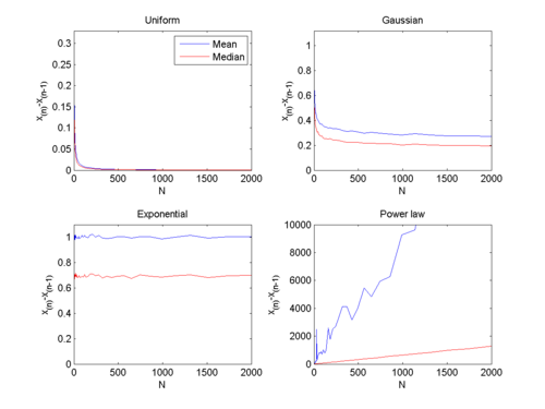
If the random numbers are uniform the the distance between the winner and the second in place is a rapidly declining function of the number of participants.A large competition will be a close one.
If the success is normally distributed, the distance is a slowly decaying function of the number of participants. Large competitions can still leave a winner far ahead.
If the success is exponentially distributed, then the average distance is constant.
If the success is power-law distributed as P(x) = Cx-2, then the distance grows linearly with the number of participants. The more participants, the more likely one is going to be to have a vast advantage.
One could of course view the random numbers as project completion times instead, and look for the minimum. This doesn't change the uniform and normal distribution cases, while the exponential and power-law cases now look much like the uniform: it doesn't take a large number of competitors to produce a small distance between the winner and second best.
The real world
In real life, project completion times are likely a mix of a Gaussian with some heavier tail for long delays, but this depends on domain. At least some project management people seem to assume something like this (scroll down). One paper found inverse Gaussian distributions at an automobile plant. PERT people appear to have a model that uses a three-point estimation to make a distribution that is kind of parabolic (I would believe this as a plot of the logarithm of probability).
Inverse Gaussians make sense, since this is the distribution of the time it takes for Brownian motion to get above a certain level if starting from 0: consider the progress of the project as Brownian, and completion times become inverse Gaussians. Here is what happens if we look at the difference between the fastest and second fastest project when their times have inverse Gaussian distributions with μ=1 and different λ (corresponding to different drift rate variabilities; high λ is close to a Gaussian):
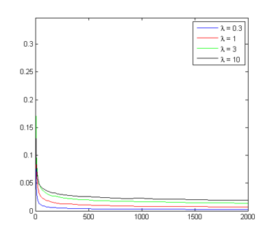
This is somewhere between the uniform case (where you are confident the project can be completed within a certain time) and a Gaussian case (there exists some unknown time when all tasks have been completed, but there are many interacting effects affecting progress). So I think this speaks in favour of numerous competitors leading to closer races, but that the winner is often noticeably far ahead, especially if the number of competitors are smaller than 10.
In real situations things become even more complex in technology races because projects may speed up or slack off as they get ahead or behind (there is a literature on this, trying to figure out the conditions when it happens). Projects may cooperate or poach ideas from each other. Ideas might float in the general milieu and produce near-simultaneous discoveries.
Proving stuff
Leaving the original question and moving towards the math: how to determine what happens as n increases?
One way of calculate it is this: The joint distribution for the n-1:th and n:th order statistics is
fX(n-1)X(n)(x,y) = n(n-1) [F(x)]n-2 f(x)f(y)
where f is the probability density function of the random variables and F is the cumulative on. So the expected difference is
E(X(n)-X(n-1)) = n(n-1) ∫ ∫x≤y (y-x) [F(x)]n-2 f(x)f(y) dx dy
Lovely little double integral that seems unlikely to budge for most distribution functions I know (sure, some transformations might work). Back to the drawing board.
Here is another rough way of estimating the behaviour:
If F is the cumulative distribution function of the random variable X, then F(X) will be uniformly distributed. The winner among n uniformly distributed variables will on average be around (n-1)/n. The second best would be around (n-2)/n. Transforming back, we get the distance between the winner and second best as:
E[X(n)-X(n-1)] = F-1((n-1)/n) - F-1((n-2)/n)
Let's try it for the exponential distribution. F(x) = 1-exp(-λ*x). F-1(y) = -(1/λ) log(1-y).
E(X(n) - X(n-1)) = (1/λ) [ -log(1-(n-1)/n) + log(1-(n-2)/n) ]
= (1/λ) log [ (1-(n-2)/n) / (1-(n-1)/n) ] = (1/λ) log(2)
Constant as n grows.
What about a power law? F(x) = 1-(x0 / x)a (a<0) (note that this a is one off from my formula in the simulation!), so F-1(y) = x0 (1-y)-1/a.
E(X(n) - X(n-1)) = x0 [ (1-(n-1)/n))-1/a - (1-(n-2)/n)-1/a ] = x0 [ n1/a - (n/2)1/a ]
If we let a=1 then the difference will grow linearly with n.
Uniform? F(x)=x, so F-1(y) =x and E(X(n) - X(n-1)) = (n-1) - (n-2) / n = 1/n.
That leaves the troublesome normal case. F(x) = 1/2 (1+erf(x/sqrt(2))). So F-1(y) = sqrt(2) erf-1 (2y-1), and we want to evaluate
E(X(n) - X(n-1)) = sqrt(2) [erf-1(2(n-1)/n-1) - erf-1(2(n-2)/n -1) ] = sqrt(2) [erf-1(1-2/n) - erf-1(1-4/n) ]
Oh joy.
Using that the derivative is (sqrt(π)/2)eerf-1(x)2 we can calculate an approximation by using the first Taylor term as E(X(n)-X(n-1)) = (sqrt(2π)/n)eerf-1(1-4/n)2. Somewhat surprisingly this actually seems to behave as the Gaussian in my simulation, but I still can't say anything about its asymptotic behaviour.
I'm not even going to try with the inverse Gaussian.
Into the library
It is said that a month in the lab can save you an hour in the library. The same is roughly true for googling things. But usually you need to dig into a problem a bit to find the right keywords to discover who already solved it long time ago.
In this case, I had rediscovered Galton's difference problem. Galton posed the question of how much of a total prize to award to the winner and to the second best in a competition, so that the second best would get a prize in proportion to their ability. (Galton, F. (1902), The Most Suitable Proportion Between The Values Of First And Second Prizes, Biometrika, 1(4), 385-390) It was solved straight away by Pearson in (Pearson, K. (1902), Note On Francis Galtons Problem, Biometrika, 1(4), 390-399.), who pioneered using order statistics to do it.
Since then people have been using this in various ways, approximating the statistics, allocating prizes and thinking of auctions, estimating confidence bounds and many other things.
In any case, the formula is
E(X(r+1)-X(r)) = [Γ(n+1)/Γ(n-r+1)Γ(r+1)] ∫ F(x)n-r[1-F(x)]r dx
Plugging in r=n-1 gives us the desired distance. Although the integral is still rather tough.
Conclusion: figuring out that what is needed is order statistics is not terribly hard. Figuring out where I can find asymptotic expressions for erf-1 near 1 is trickier. We need to have a maths concept search engine!
(Incidentally, those early issues of Biometrika were cool. Smallpox vaccination, life expectancies of mummies, new statistical concepts, skull measurements, all mixed together.)