 Continuing my intermittent Newtonmas fractal tradition (2014, 2016, 2018), today I play around with a very suitable fractal based on gravity.
The problem
On Physics StackExchange NiveaNutella asked a simple yet tricky to answer question:
If we have two unmoving equal point masses in the plane (let’s say at ")
User Kasper showed that one can reframe the problem in terms of elliptic coordinates and show that this implies a straight boundary, while User Lineage showed it more simply using the second constant of motion. I have the feeling that there ought to be an even simpler argument. Still, Kasper’s solution show that the generic trajectory will quasiperiodically fill a region and tend to come arbitrarily close to one of the masses.
The fractal
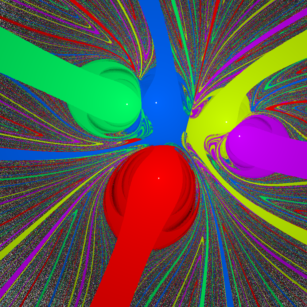
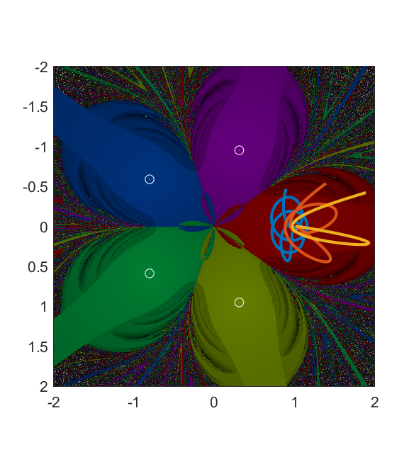
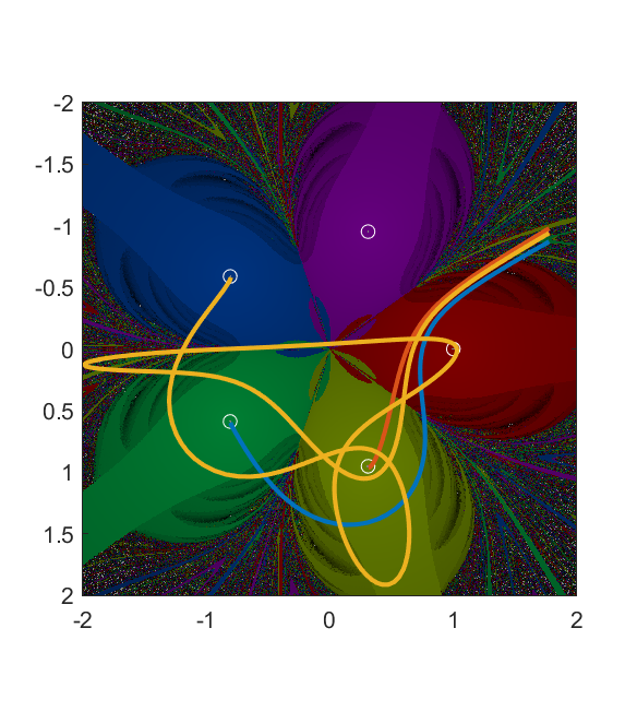
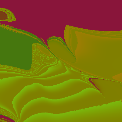
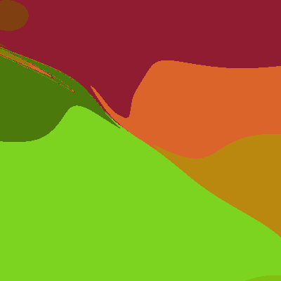
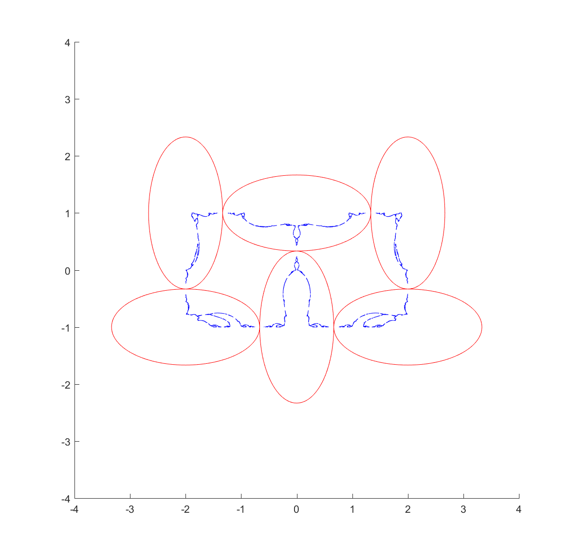
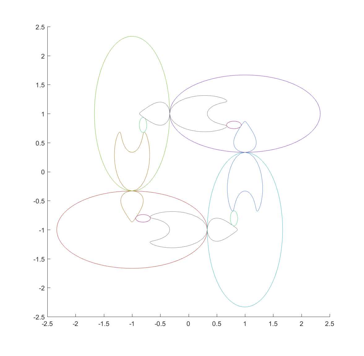
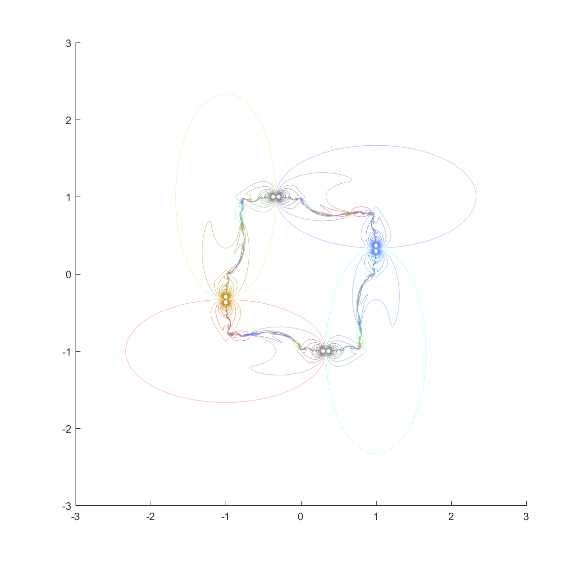
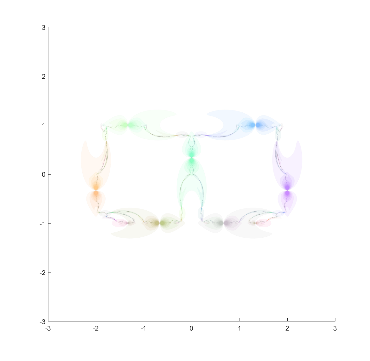
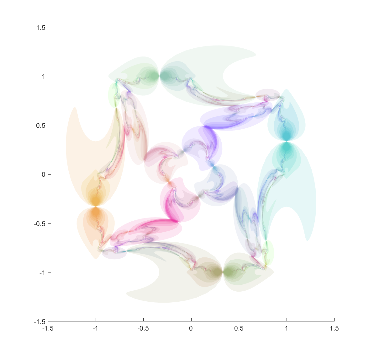
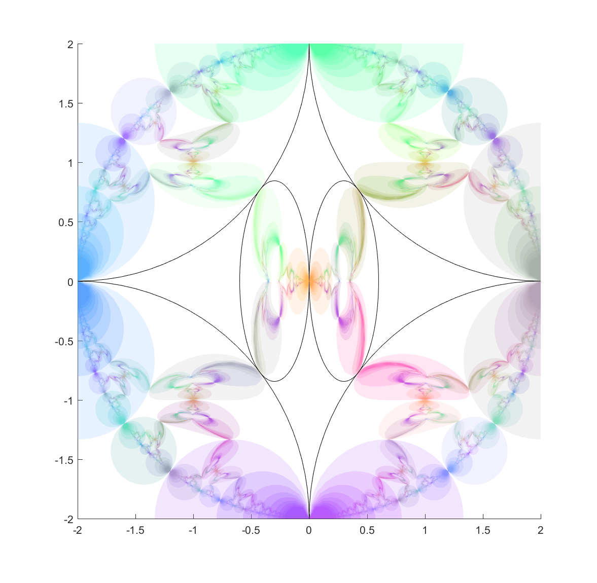
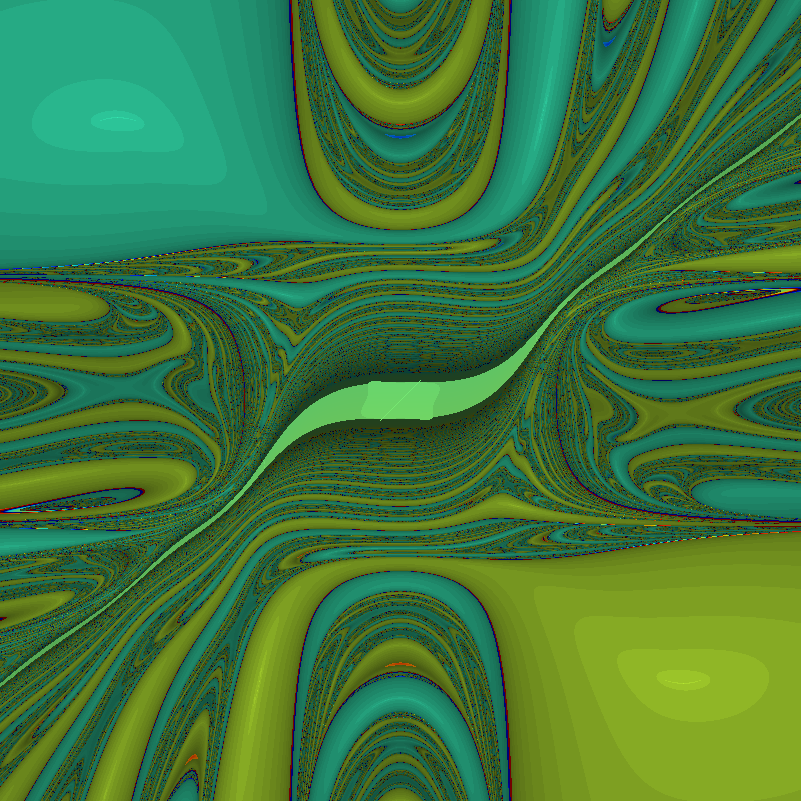
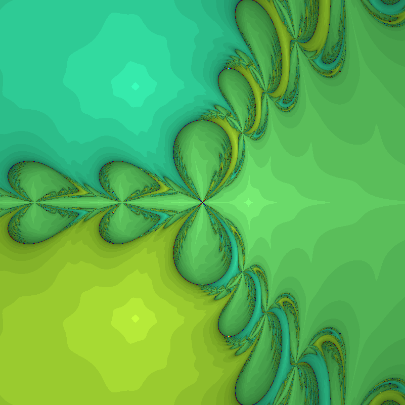
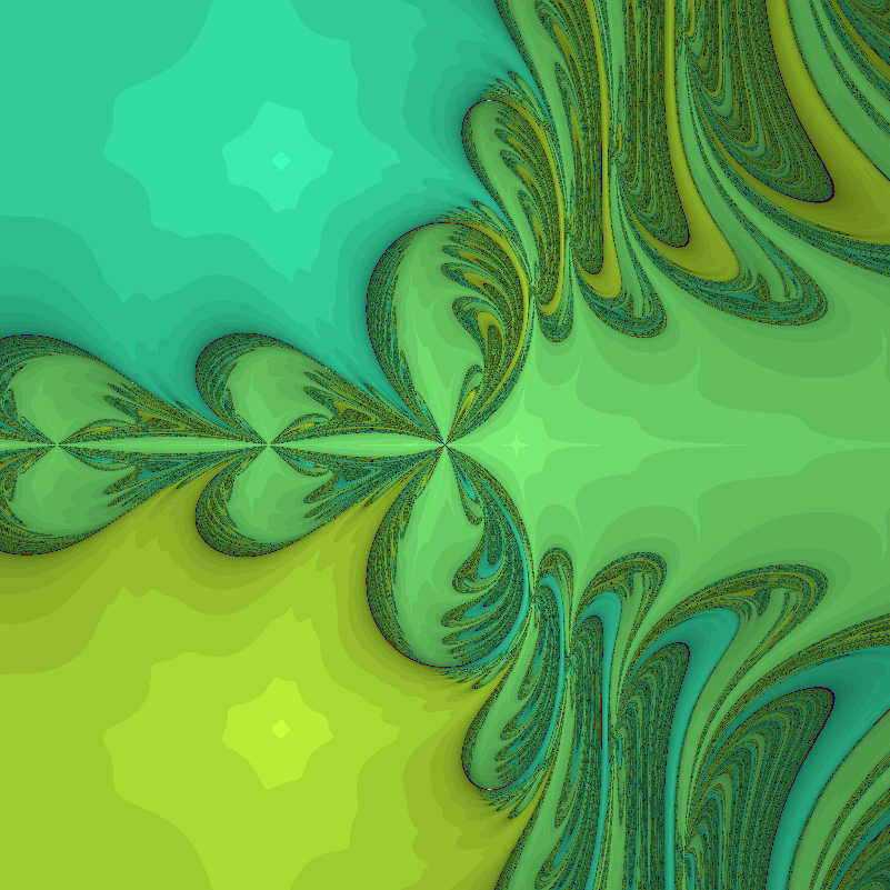
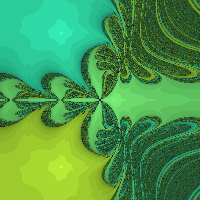
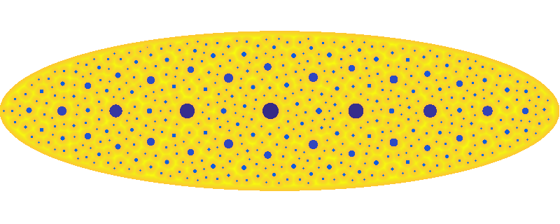
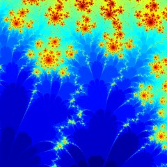
In any case, here is a plot of the basins of attraction shaded by the time until getting within a small radius 
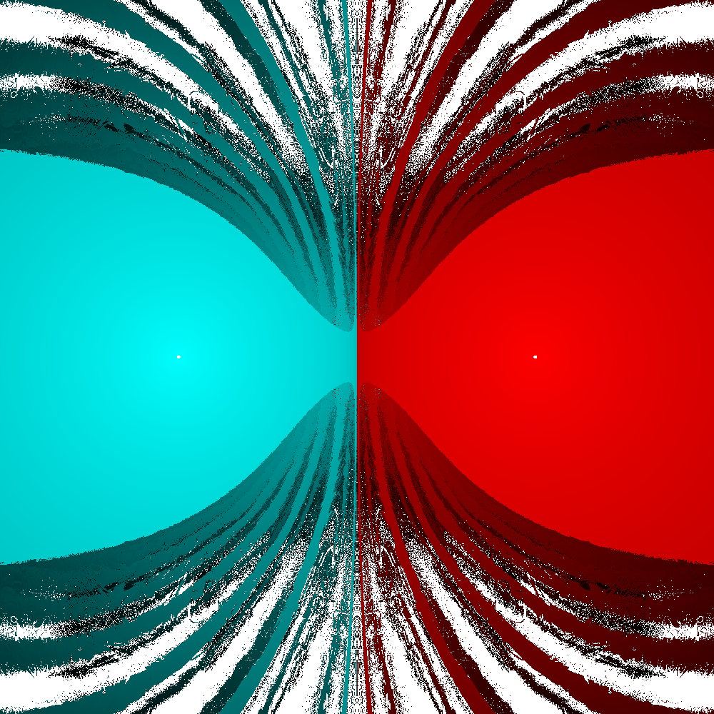
The boundary is a straight line, and surrounding the simple regions where orbits fall nearly straight into the nearest mass are the wilder regions where orbits first rock back and forth across the x-axis before settling into ellipses around the masses.
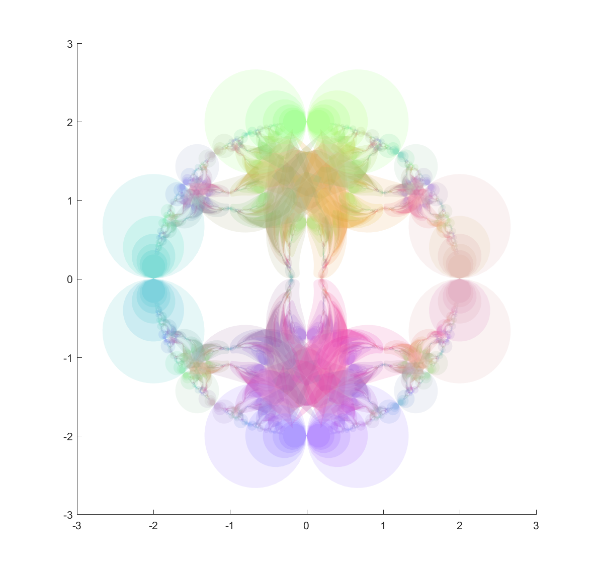
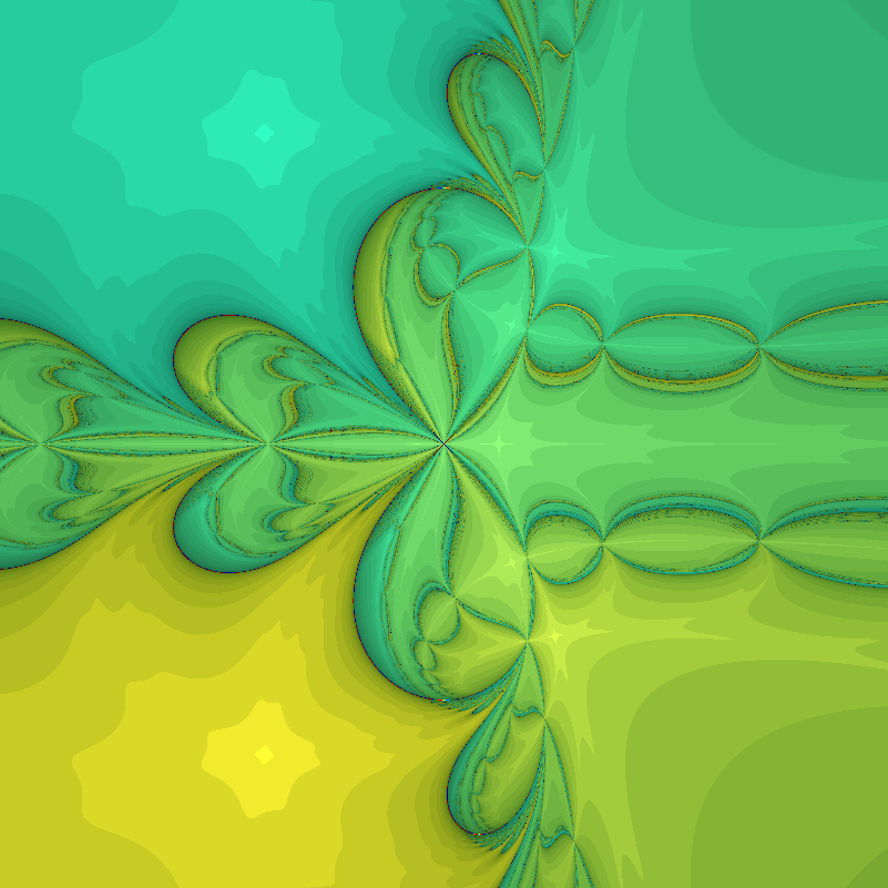
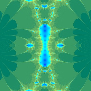
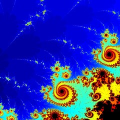
The case for 5 evenly spaced masses for 

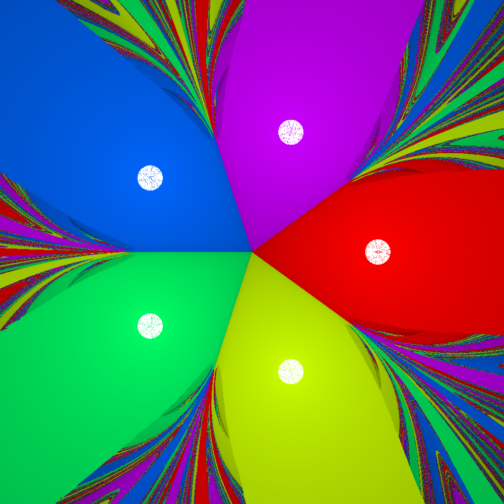

As 
I cannot claim credit for this fractal, as NiveaNutella already plotted it. But it still fascinates me.

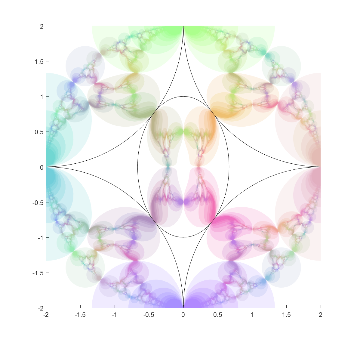
Wada basins and mille-feuille collision manifolds
These patterns are somewhat reminiscent of the classic Newton’s root-finding iterative formula fractals: several basins of attraction with a fractal border where pairs of basins encounter interleaved tiny parts of basins not member of the pair.
However, this dynamics is continuous rather than discrete. The plane is a 2D section through a 4D phase space, where starting points at zero velocity accelerate so that they bob up and down/ana and kata along the velocity axes. This also leads to a neat property of the basins of attraction: they are each arc-connected sets, since for any two member points that are the start of trajectories they end up in a small ball around the attractor mass. One can hence construct a map from ![[0,1]](https://s0.wp.com/latex.php?latex=%5B0%2C1%5D&bg=ffffff&fg=000000&s=0 "[0,1]")
")
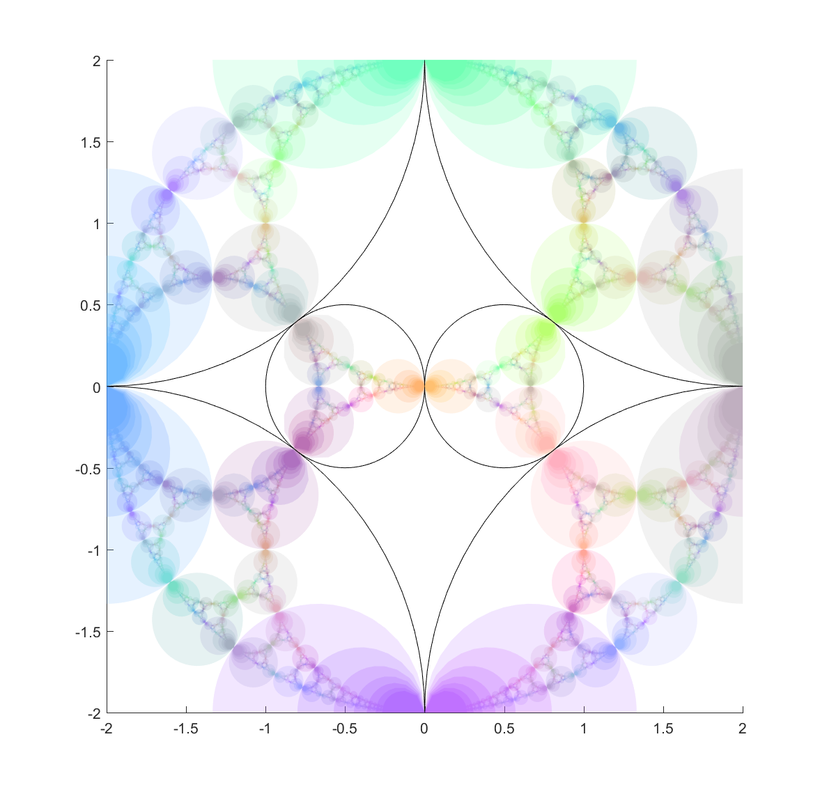
Each mass is surrounded by a set of trajectories hitting it exactly, which we can parametrize by the angle they make and the speed they have inwards when they pass some circle around the mass point. They hence form a 3D manifold 
")


The magnetic pendulum
This fractal is similar to one I made back in 1990 inspired by the dynamics of the magnetic decision-making desk toy, a pendulum oscillating above a number of magnets. Eventually it settles over one. The basic dynamics is fairly similar (see Zhampres’ beautiful images or this great treatment). The difference is that the gravity fractal has no dissipation: in principle orbits can continue forever (but I end when they get close to the masses or after a timeout) and in the magnetic fractal the force dependency was bounded, a ")

That simulation was part of my epic third year project in the gymnasium. The topic was “Chaos and self-organisation”, and I spent a lot of time reading the dynamical systems literature, running computer simulations, struggling with WordPerfect’s equation editor and producing a manuscript of about 150 pages that required careful photocopying by hand to get the pasted diagrams on separate pieces of paper to show up right. My teacher eventually sat down with me and went through my introduction and had me explain Poincaré sections. Then he promptly passed me. That was likely for the best for both of us.
Appendix: Matlab code
showPlot=0; % plot individual trajectories
randMass = 0; % place masses randomly rather than in circle

RTRAP=0.0001; % size of trap region
tmax=60; % max timesteps to run
S=1000; % resolution

x=linspace(-2,2,S);
y=linspace(-2,2,S);
[X,Y]=meshgrid(x,y);

N=5;
theta=(0:(N-1))*pi*2/N;
PX=cos(theta); PY=sin(theta);
if (randMass==1)
s = rng(3);
PX=randn(N,1); PY=randn(N,1);
end

clf

hit=X*0;
hitN = X*0; % attractor basin
hitT = X*0; % time until hit
closest = X*0+100;
closestN=closest; % closest mass to trajectory

tic; % measure time
for a=1:size(X,1)
disp(a)
for b=1:size(X,2)
[t,u,te,ye,ie]=ode45(@(t,y) forceLaw(t,y,N,PX,PY), [0 tmax], [X(a,b) 0 Y(a,b) 0],odeset('Events',@(t,y) finishFun(t,y,N,PX,PY,RTRAP^2)));

if (showPlot==1)
plot(u(:,1),u(:,3),'-b')
hold on
end

if (~isempty(te))
hit(a,b)=1;
hitT(a,b)=te;

mind2=100^2;
for k=1:N
dx=ye(1)-PX(k);
dy=ye(3)-PY(k);
d2=(dx.^2+dy.^2);
if (d2<mind2) mind2=d2; hitN(a,b)=k; end
end

end
for k=1:N
dx=u(:,1)-PX(k);
dy=u(:,3)-PY(k);
d2=min(dx.^2+dy.^2);
closest(a,b)=min(closest(a,b),sqrt(d2));

if (closest(a,b)==sqrt(d2)) closestN(a,b)=k; end
end
end

if (showPlot==1)
drawnow
pause
end
end
elapsedTime = toc

if (showPlot==0)
% Make colorful plot
co=hsv(N);
mag=sqrt(hitT);
mag=1-(mag-min(mag(:)))/(max(mag(:))-min(mag(:)));
im=zeros(S,S,3);
im(:,:,1)=interp1(1:N,co(:,1),closestN).*mag;
im(:,:,2)=interp1(1:N,co(:,2),closestN).*mag;
im(:,:,3)=interp1(1:N,co(:,3),closestN).*mag;
image(im)
end

% Gravity
function dudt = forceLaw(t,u,N,PX,PY)
%dudt = zeros(4,1);
dudt=u;
dudt(1) = u(2);
dudt(2) = 0;
dudt(3) = u(4);
dudt(4) = 0;

dx=u(1)-PX;
dy=u(3)-PY;
d=(dx.^2+dy.^2).^-1.5;
dudt(2)=dudt(2)-sum(dx.*d);
dudt(4)=dudt(4)-sum(dy.*d);

% for k=1:N
% dx=u(1)-PX(k);
% dy=u(3)-PY(k);
% d=(dx.^2+dy.^2).^-1.5;
% dudt(2)=dudt(2)-dx.*d;
% dudt(4)=dudt(4)-dy.*d;
% end
end

% Are we close enough to one of the masses?
function [value,isterminal,direction] =finishFun(t,u,N,PX,PY,r2)
value=1000;
for k=1:N
dx=u(1)-PX(k);
dy=u(3)-PY(k);
d2=(dx.^2+dy.^2);
value=min(value, d2-r2);
end
isterminal=1;
direction=0;
end
 to find a better approximation
 /f'(z_{n})") . This will work as long as
. This will work as long as \neq 0") , but which root one converges to can be sensitively dependent on initial conditions. Plotting which root a given initial value ends up with gives the Newton fractal.
, but which root one converges to can be sensitively dependent on initial conditions. Plotting which root a given initial value ends up with gives the Newton fractal.=\sum_{i=1}^m r_i^2(\beta)") when some function dependent on n-dimensional parameters $\beta$ is fitted to
when some function dependent on n-dimensional parameters $\beta$ is fitted to  data points
 =f(x_i;\beta)-y_i") . Just like the root finding method it iterates towards a minimum of
. Just like the root finding method it iterates towards a minimum of ") :
: ^{-1}J^t r(\beta)") where
where  is the Jacobian
  . This is essentially Newton’s method but in a multi-dimensional form.
![f(x;\beta_1,\beta_2)=(1/\sqrt{2\pi})[e^{-(x-\beta_1)^2/2}+(1/4)e^{-(x-\beta_1)^2/8}]](https://s0.wp.com/latex.php?latex=f%28x%3B%5Cbeta_1%2C%5Cbeta_2%29%3D%281%2F%5Csqrt%7B2%5Cpi%7D%29%5Be%5E%7B-%28x-%5Cbeta_1%29%5E2%2F2%7D%2B%281%2F4%29e%5E%7B-%28x-%5Cbeta_1%29%5E2%2F8%7D%5D&bg=ffffff&fg=000000&s=0 "f(x;\beta_1,\beta_2)=(1/\sqrt{2\pi})[e^{-(x-\beta_1)^2/2}+(1/4)e^{-(x-\beta_1)^2/8}]") (one Gaussian with variance 1 and one with 1/4 – the reason for this is not to make the diagram boringly symmetric as for the same variance case). Plotting the location of the final
(one Gaussian with variance 1 and one with 1/4 – the reason for this is not to make the diagram boringly symmetric as for the same variance case). Plotting the location of the final ") (by stereographically mapping it onto a unit sphere in (r,g,b) space) gives a nice fractal:
(by stereographically mapping it onto a unit sphere in (r,g,b) space) gives a nice fractal: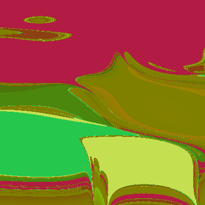
=0") for some n) with different basins alternating.
for some n) with different basins alternating.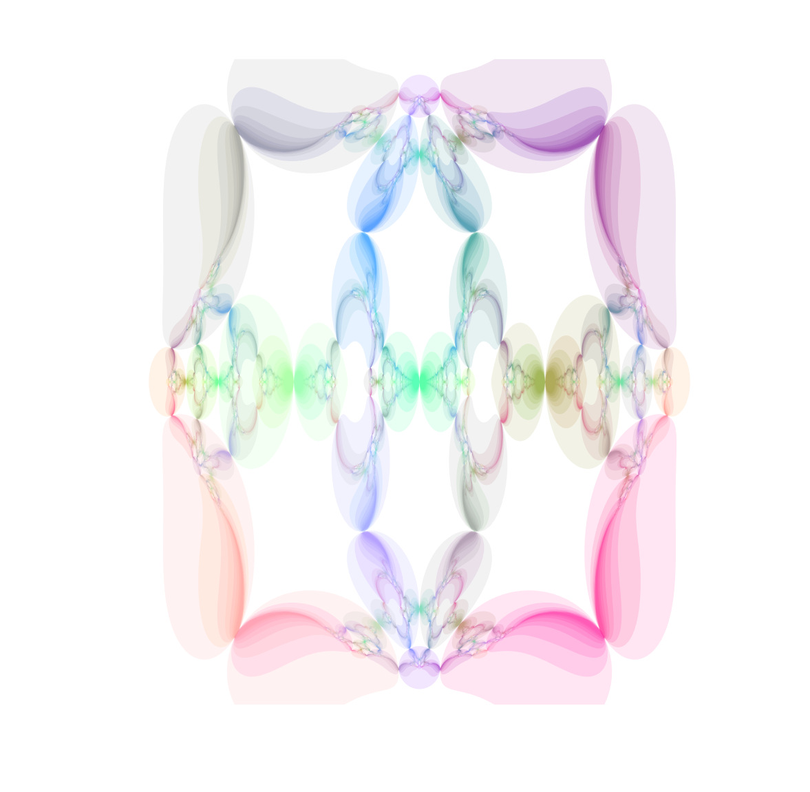
 is projected to another point
  so that
  where
where  is the centre of the ellipse and
  is the point where the ray between
  intersects the ellipse.
 , the inverse point of
 ") is
is ") where
where  and
and  . Basically this is a squashed version of the circle formula.
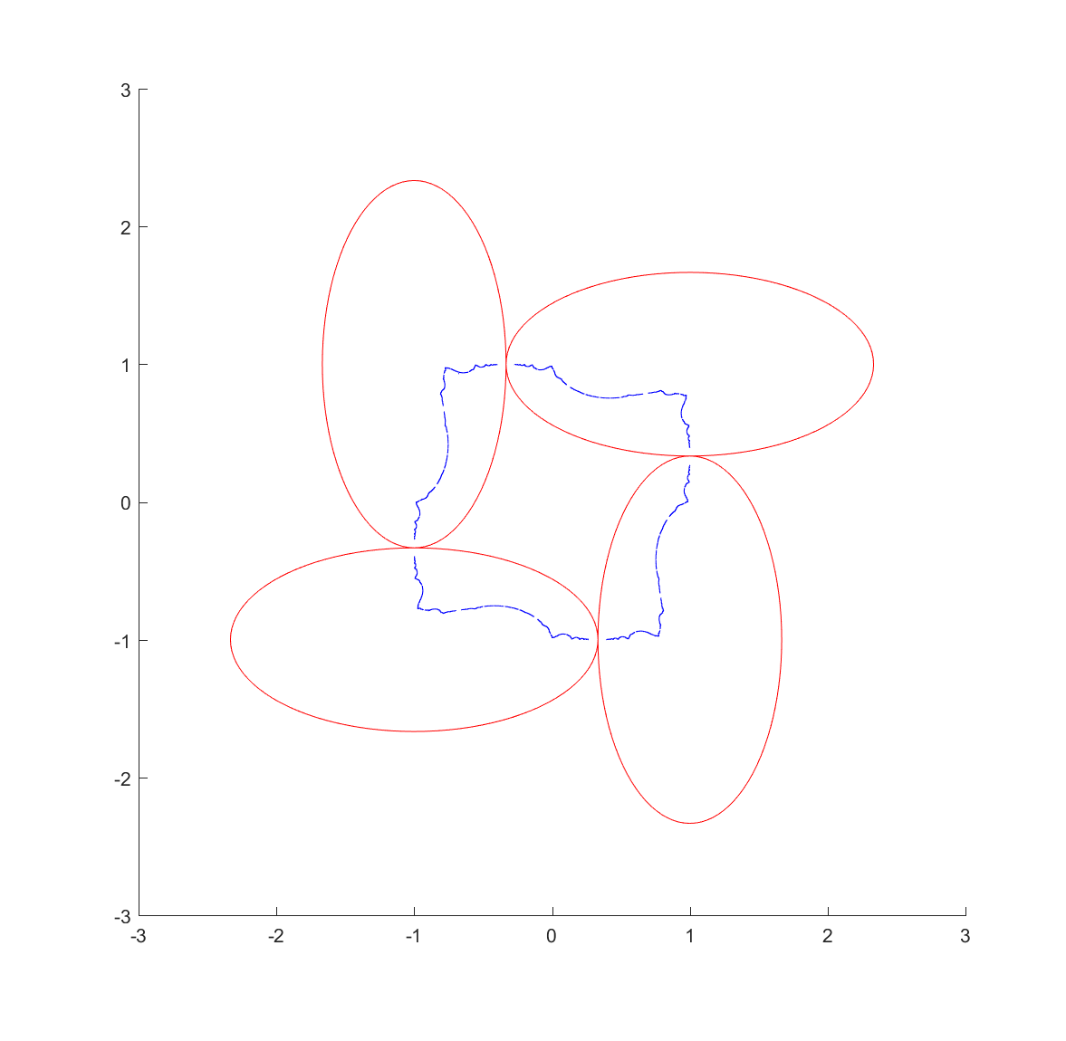
 to
to ![[\tanh(x),\tanh(y)]](https://s0.wp.com/latex.php?latex=%5B%5Ctanh%28x%29%2C%5Ctanh%28y%29%5D&bg=ffffff&fg=000000&s=0 "[\tanh(x),\tanh(y)]") . The origin is unchanged, and infinity becomes the edges of the square
. The origin is unchanged, and infinity becomes the edges of the square ![[-1,1]\times [-1,1]](https://s0.wp.com/latex.php?latex=%5B-1%2C1%5D%5Ctimes+%5B-1%2C1%5D&bg=ffffff&fg=000000&s=0 "[-1,1]\times [-1,1]") . This is not a conformal map, so things will get squished near the edges.
. This is not a conformal map, so things will get squished near the edges.![(1/2)+(1/2)[\tanh(|z-1|-1), \tanh(|z+1|-1), \tanh(|z-i|-1)]](https://s0.wp.com/latex.php?latex=%281%2F2%29%2B%281%2F2%29%5B%5Ctanh%28%7Cz-1%7C-1%29%2C+%5Ctanh%28%7Cz%2B1%7C-1%29%2C+%5Ctanh%28%7Cz-i%7C-1%29%5D&bg=ffffff&fg=000000&s=0 "(1/2)+(1/2)[\tanh(|z-1|-1), \tanh(|z+1|-1), \tanh(|z-i|-1)]") to map complex coordinates to RGB. This makes the color depend on the distance to 1, -1 and i, making infinity white and zero some drab color (the -1 terms at the end determines the overall color range).
to map complex coordinates to RGB. This makes the color depend on the distance to 1, -1 and i, making infinity white and zero some drab color (the -1 terms at the end determines the overall color range). where
where  is independent random numbers is a
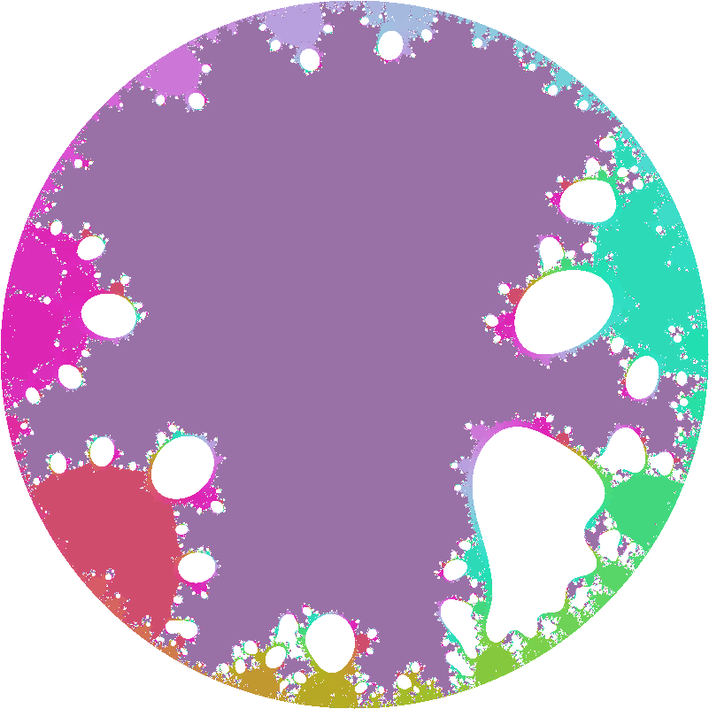

 fractal every point on the boundary is a meeting point of the three basins, a
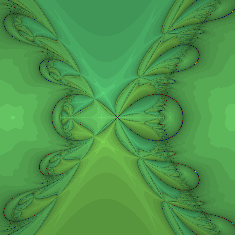
") the zeros will typically form a curve in the plane. In order to get discrete zeros we typically need to have two functions to produce a zero set. We can think of it as a map from R2 to R2
the zeros will typically form a curve in the plane. In order to get discrete zeros we typically need to have two functions to produce a zero set. We can think of it as a map from R2 to R2 ![F(x)=[f_1(x_1,x_2), f_2(x_1,x_2)]](https://s0.wp.com/latex.php?latex=F%28x%29%3D%5Bf_1%28x_1%2Cx_2%29%2C+f_2%28x_1%2Cx_2%29%5D+&bg=ffffff&fg=000000&s=0 "F(x)=[f_1(x_1,x_2), f_2(x_1,x_2)]") where the x’es are 2D vectors. In this case Newton’s method turns into solving the linear equation system
where the x’es are 2D vectors. In this case Newton’s method turns into solving the linear equation system (x_{n+1}-x_n)=-F(x_n)") where
where ") is the Jacobian matrix (
is the Jacobian matrix ( ) and
) and  now denotes the n’th iterate.
![F=[x^3-x-y, y^3-x-y]](https://s0.wp.com/latex.php?latex=F%3D%5Bx%5E3-x-y%2C+y%5E3-x-y%5D&bg=ffffff&fg=000000&s=0 "F=[x^3-x-y, y^3-x-y]") . Below is a plot of the first and second components (red and green), as well as a blue plane for zero values. The zeros of the function are the three points where red, green and blue meet.
. Below is a plot of the first and second components (red and green), as well as a blue plane for zero values. The zeros of the function are the three points where red, green and blue meet. , one at
  , and one at
  The middle one has a region of troublesomely similar function values – the red and green surfaces are tangent there.
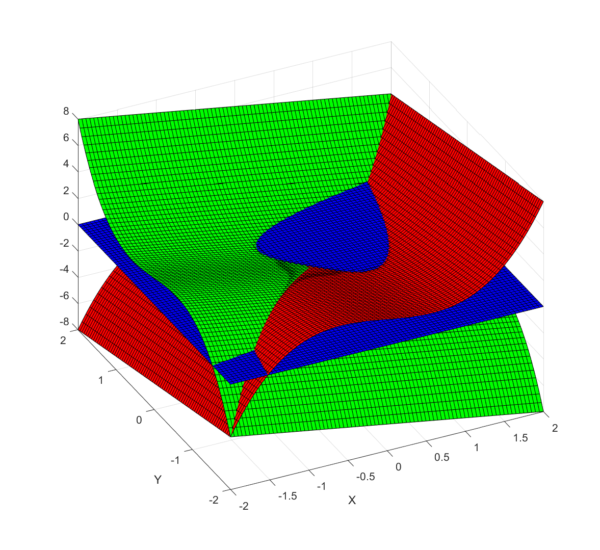
![Behavior of Newton's method in 2D for F=[x^3-x-y, y^3-x-y]. Color denotes value of x+y, with darkening for slow convergence.](http://aleph.se/andart2/wp-content/uploads/2016/12/newton2dp1.png)
 (where
  and
and  if the matrix has the usual
 ![[a b; c d]](https://s0.wp.com/latex.php?latex=%5Ba+b%3B+c+d%5D&bg=ffffff&fg=000000&s=0 "[a b; c d]") form). So if the trace and determinant are randomly chosen, we should expect a majority of cases to be non-rotational.
form). So if the trace and determinant are randomly chosen, we should expect a majority of cases to be non-rotational.![F=[x \cos(\theta) + y \sin(\theta), x\sin(\theta)+y\cos(\theta)]](https://s0.wp.com/latex.php?latex=F%3D%5Bx+%5Ccos%28%5Ctheta%29+%2B+y+%5Csin%28%5Ctheta%29%2C+x%5Csin%28%5Ctheta%29%2By%5Ccos%28%5Ctheta%29%5D&bg=ffffff&fg=000000&s=0 "F=[x \cos(\theta) + y \sin(\theta), x\sin(\theta)+y\cos(\theta)]") . This is of course just a rotation by the angle theta, and it does not have very interesting zeros.
. This is of course just a rotation by the angle theta, and it does not have very interesting zeros. \cos(\theta)")
 \sin(\theta),")
![(x^3-x-y) \sin(\theta)+(y^3-y-x) \cos(\theta) ]](https://s0.wp.com/latex.php?latex=%28x%5E3-x-y%29+%5Csin%28%5Ctheta%29%2B%28y%5E3-y-x%29+%5Ccos%28%5Ctheta%29+%5D&bg=ffffff&fg=000000&s=0 "(x^3-x-y) \sin(\theta)+(y^3-y-x) \cos(\theta) ]") . The result is fun, but still far from baroque:
. The result is fun, but still far from baroque: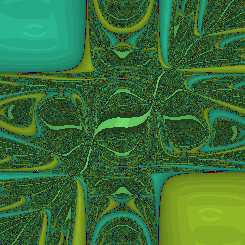
 to make the dynamics even more complex:
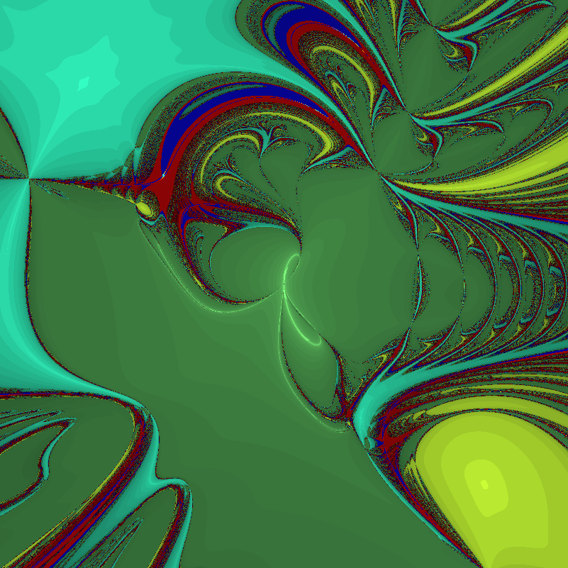
![F=[x^3-3xy^2-1, 3x^2y-y^3]](https://s0.wp.com/latex.php?latex=F%3D%5Bx%5E3-3xy%5E2-1%2C+3x%5E2y-y%5E3%5D&bg=ffffff&fg=000000&s=0 "F=[x^3-3xy^2-1, 3x^2y-y^3]") (which produces the archetypal
(which produces the archetypal =z^3-1") Newton fractal).
Newton fractal).![Newton fractal for F=[x^3-3xy^2-1, 3x^2y-y^3].](http://aleph.se/andart2/wp-content/uploads/2016/12/newtonpert0.png)
![F=[x^3-3xy^2-1 + \epsilon x, 3x^2y-y^3]](https://s0.wp.com/latex.php?latex=F%3D%5Bx%5E3-3xy%5E2-1+%2B+%5Cepsilon+x%2C+3x%5E2y-y%5E3%5D&bg=ffffff&fg=000000&s=0 "F=[x^3-3xy^2-1 + \epsilon x, 3x^2y-y^3]") , then for
, then for  we get:
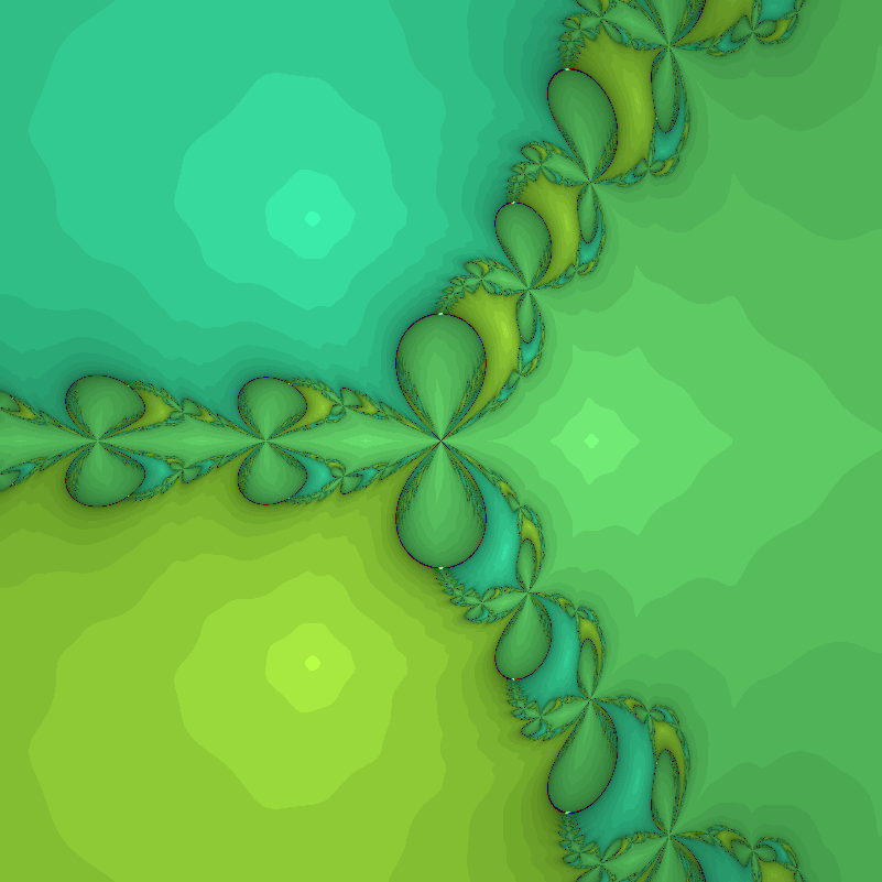
 at the point with maximal distance
 ") from the border.
from the border.") , which is then updated
, which is then updated  \leftarrow \min(d(x,y), D(x,y))") where
where ") is the distance to the circle. This trades exactness for some discretization error, but it can easily handle nearly arbitrary shapes.
is the distance to the circle. This trades exactness for some discretization error, but it can easily handle nearly arbitrary shapes.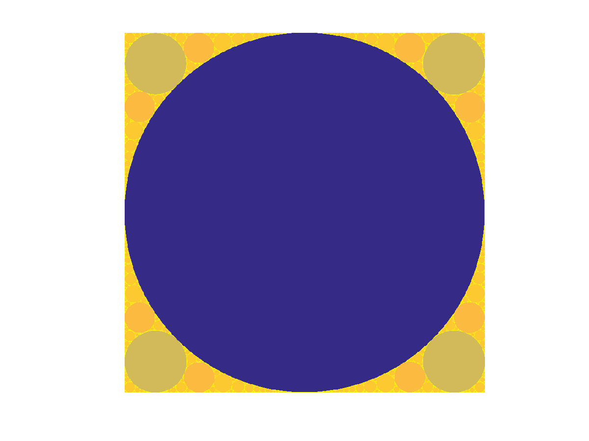
 .
.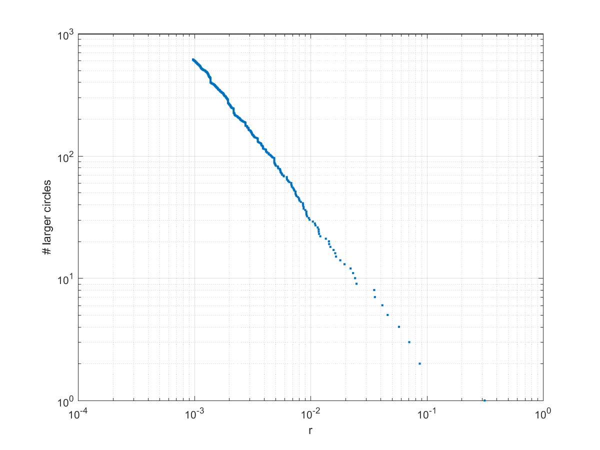
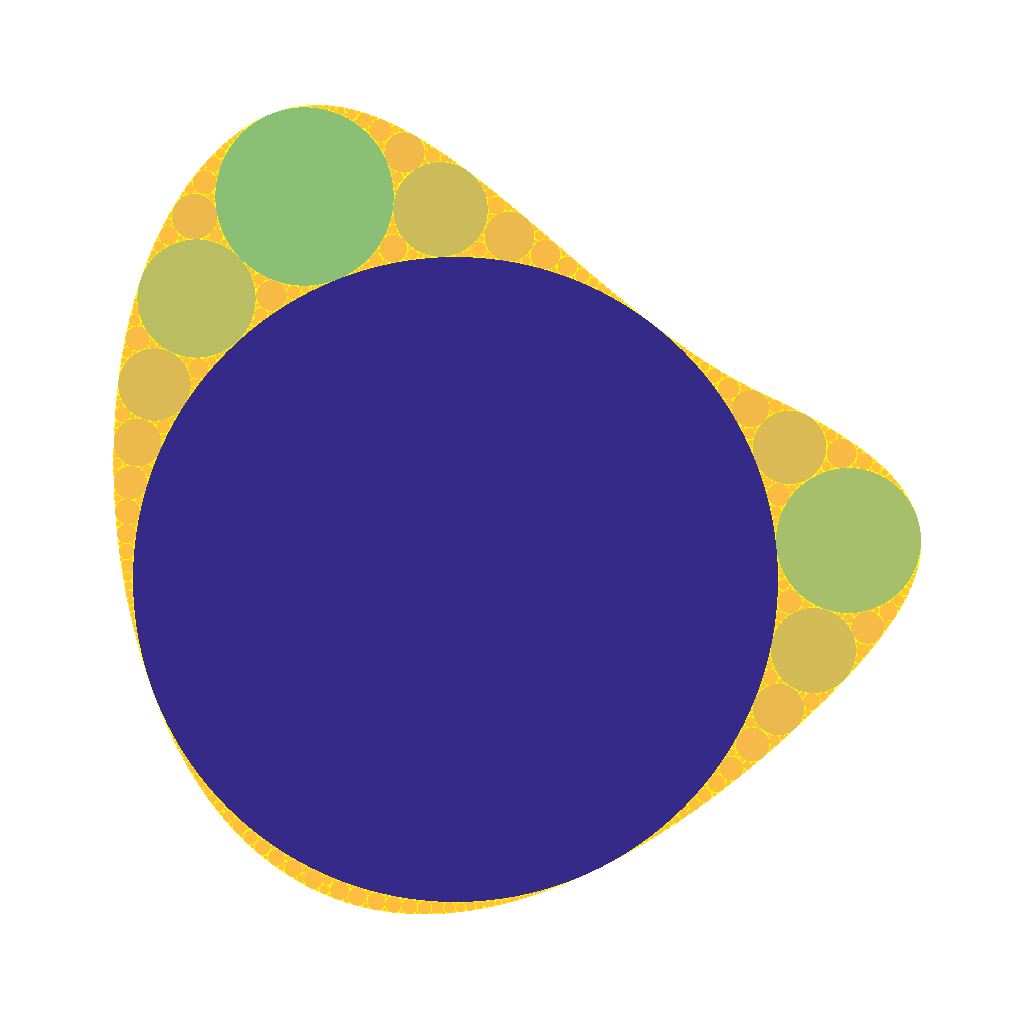
\propto r^-\delta") as we approach zero, with
as we approach zero, with  . This is unsurprising: given a generic curved triangle, the inscribed circle will be a fraction of the radii of the bordering circles. If one looks at
  is the Hausdorff dimension of the gasket.
 .
.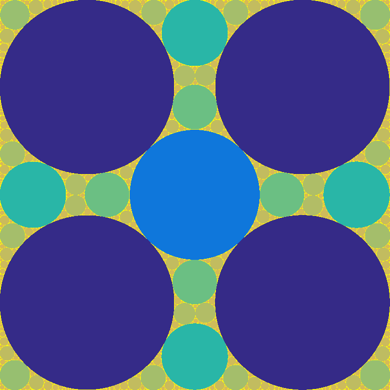
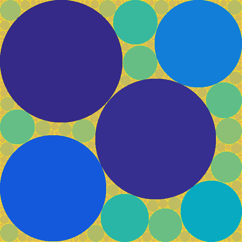
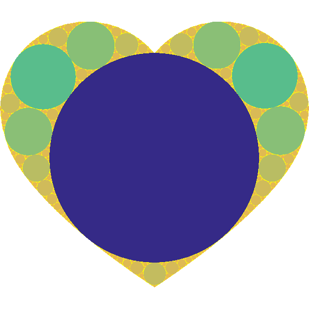
 we get sponge-like fractals: these are relatives to the Menger sponge and the Cantor set. The domain gets an infinity of circles punched out of itself, with a total area approaching the area of the domain, so the total measure goes to zero.

=\int_0^\infty t^{z-1}e^{-t} dt") , the continuous generalization of the factorial. While it grows rapidly for positive reals, it has fun poles for the negative integers and is generally complex.
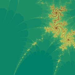
, the continuous generalization of the factorial. While it grows rapidly for positive reals, it has fun poles for the negative integers and is generally complex. ") . The result is a nice fractal, with some domains approaching 1, and others running off to infinity.
. The result is a nice fractal, with some domains approaching 1, and others running off to infinity.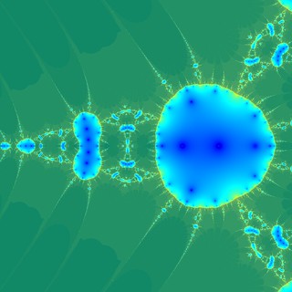
 . Zooming in a bit more reveals neat self-similar patterns with alternating “beans”:
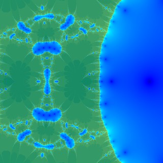
") where c is the control parameter. I start with
where c is the control parameter. I start with  and iterate:
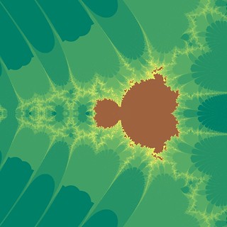
 has an infinite decimal expansion, does that mean the collected works of Shakespeare (suitably encoded) are in it somewhere?”
 is a Shakespeare-free number (unless we have a bizarre encoding of the works in the form of all threes). What really matters is whether the number is suitably random. In mathematics this is known as the question about whether pi is a
 ![[Shakespeare]](https://s0.wp.com/latex.php?latex=%5BShakespeare%5D&bg=ffffff&fg=000000&s=0 "[Shakespeare]") , all numbers of the form
, all numbers of the form ![0.[Shakespeare]xxxxx\ldots](https://s0.wp.com/latex.php?latex=0.%5BShakespeare%5Dxxxxx%5Cldots+&bg=ffffff&fg=000000&s=0 "0.[Shakespeare]xxxxx\ldots") are Shakespeare-containing.
are Shakespeare-containing.![[0. 527269000\ldots , 0.52727]](https://s0.wp.com/latex.php?latex=%5B0.+527269000%5Cldots+%2C+0.52727%5D&bg=ffffff&fg=000000&s=0 "[0. 527269000\ldots , 0.52727]") , a mere millionth of
, a mere millionth of ![0.y[Shakespeare]xxxx\ldots](https://s0.wp.com/latex.php?latex=0.y%5BShakespeare%5Dxxxx%5Cldots+&bg=ffffff&fg=000000&s=0 "0.y[Shakespeare]xxxx\ldots") , where
, where  is a digit different from the starting digit of
  anything else. So there are 9 such second level intervals, each ten times thinner than the first level interval.
![[Shakespeare]=3](https://s0.wp.com/latex.php?latex=%5BShakespeare%5D%3D3&bg=ffffff&fg=000000&s=0 "[Shakespeare]=3") , so all numbers containing the digit 3 in the decimal expansion are Shakespearian and the rest are Shakespeare-free.
, so all numbers containing the digit 3 in the decimal expansion are Shakespearian and the rest are Shakespeare-free.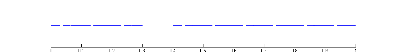
/\log(10)\approx 0.9542") . This is less than 1: most points are Shakespearian and in one of the intervals, but since they are thin compared to the line the Shakespeare-free set is nearly one dimensional. Like the Cantor set, each Shakespeare-free number is isolated from any other Shakespeare-free number: there is always some Shakespearian numbers between them.
. This is less than 1: most points are Shakespearian and in one of the intervals, but since they are thin compared to the line the Shakespeare-free set is nearly one dimensional. Like the Cantor set, each Shakespeare-free number is isolated from any other Shakespeare-free number: there is always some Shakespearian numbers between them. . The fractal dimension of the Shakespeare-free set is
 /\log(10^{10,600,600}) \approx 1-\epsilon") , for some tiny
, for some tiny  . It is very nearly an unbroken line… except for that nearly every point actually does contain Shakespeare.
![[Shakespeare][Shakespeare]xxx\ldots](https://s0.wp.com/latex.php?latex=%5BShakespeare%5D%5BShakespeare%5Dxxx%5Cldots&bg=ffffff&fg=000000&s=0 "[Shakespeare][Shakespeare]xxx\ldots") numbers…
numbers… of being in the level 1 interval of Shakespearian numbers. If not, then it will be in one of the 9 intervals 1/10 long that don’t start with the correct first digit, where the probability of starting with Shakespeare in the second digit is
 S+(9/10^2)S+\ldots = 10S<1") . But the 1/10 interval around the first Shakespearian interval also counts: a number that has the right first digit but wrong second digit can still be Shakespearian. So it will add probability.
. But the 1/10 interval around the first Shakespearian interval also counts: a number that has the right first digit but wrong second digit can still be Shakespearian. So it will add probability.S") (the first factor is the probability of not having Shakespeare first), and so on. So the total probability of finding Shakespeare is
(the first factor is the probability of not having Shakespeare first), and so on. So the total probability of finding Shakespeare is S + (1-S)^2S + (1-S)^3S + \ldots = S/(1-(1-S))=1") . So nearly all numbers are Shakespearian.
. So nearly all numbers are Shakespearian.![0.[Shakespeare]000\ldots](https://s0.wp.com/latex.php?latex=0.%5BShakespeare%5D000%5Cldots+&bg=ffffff&fg=000000&s=0 "0.[Shakespeare]000\ldots") is non-normal but Shakespearian. So is
is non-normal but Shakespearian. So is ![0.[Shakespeare][Shakespeare][Shakespeare]\ldots](https://s0.wp.com/latex.php?latex=0.%5BShakespeare%5D%5BShakespeare%5D%5BShakespeare%5D%5Cldots+&bg=ffffff&fg=000000&s=0 "0.[Shakespeare][Shakespeare][Shakespeare]\ldots") We can throw in arbitrary finite sequences of digits between the Shakespeares, biasing numbers as close or far as we want from normality. There is a number
We can throw in arbitrary finite sequences of digits between the Shakespeares, biasing numbers as close or far as we want from normality. There is a number ![0.[Shakespeare]3141592\ldots](https://s0.wp.com/latex.php?latex=0.%5BShakespeare%5D3141592%5Cldots&bg=ffffff&fg=000000&s=0 "0.[Shakespeare]3141592\ldots") that has the digits of
that has the digits of 
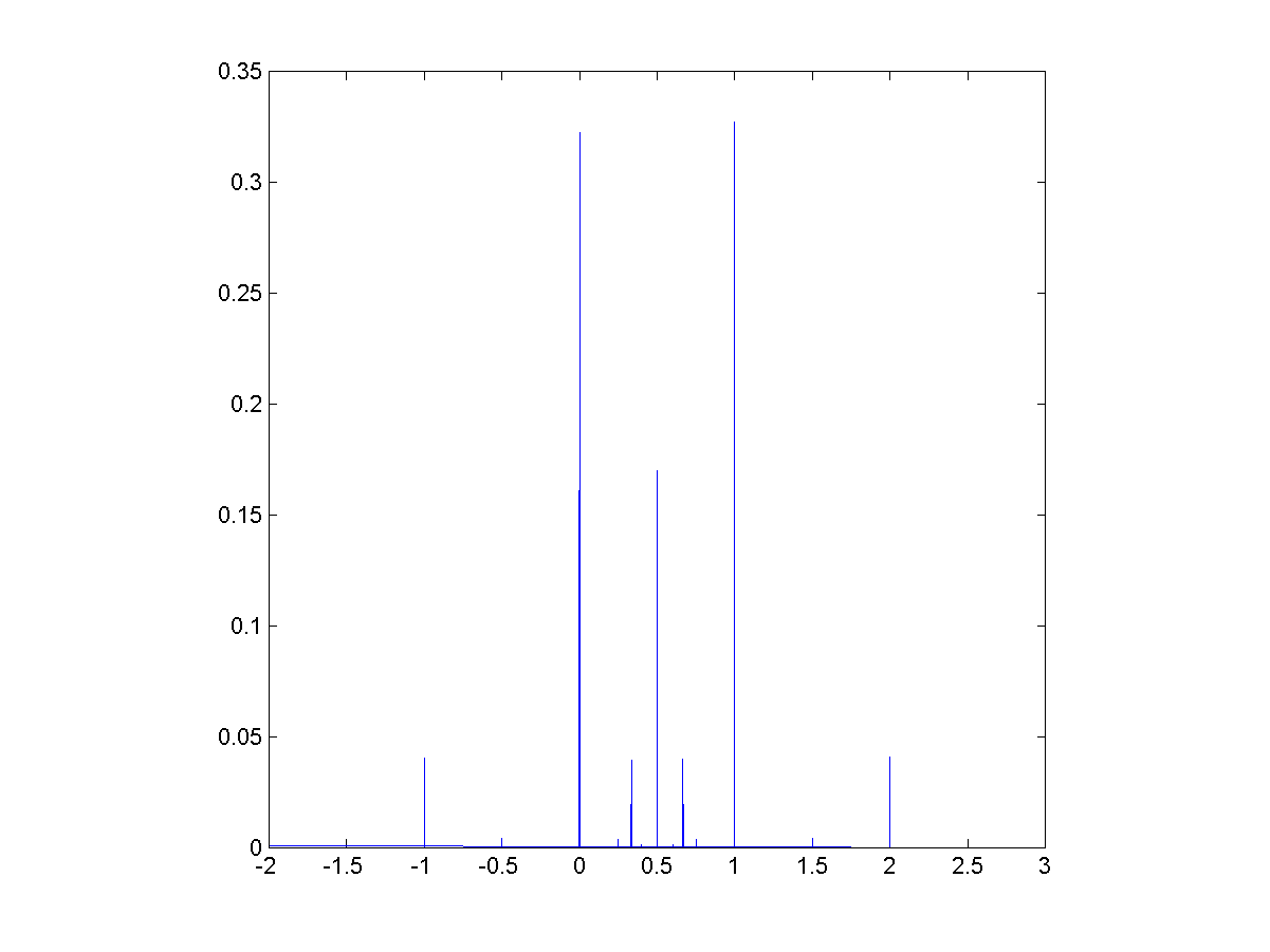
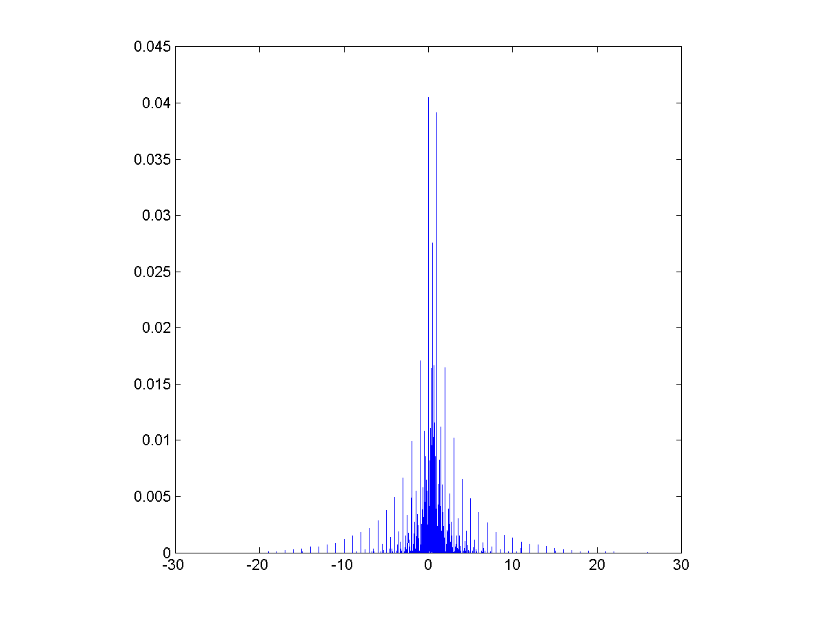
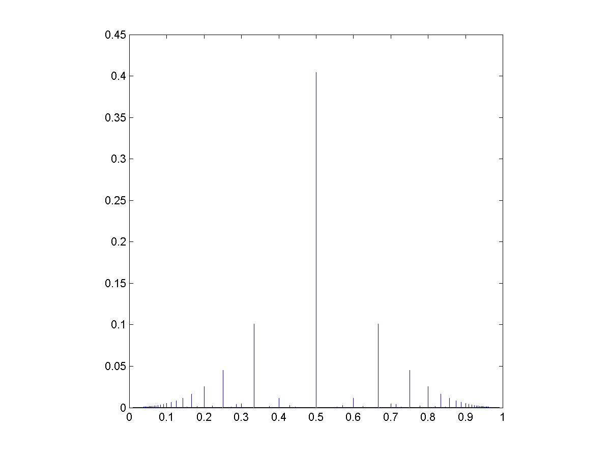
") and generate ratios
and generate ratios ") , then those ratios will have a distribution that is a convolution over the rational numbers:
, then those ratios will have a distribution that is a convolution over the rational numbers:  = g(a/(a+b)) = \sum_{m=0}^\infty \sum_{n=0}^\infty f(m) g(n) \delta \left(\frac{a}{a+b} - \frac{m}{m+n} \right ) = \sum_{t=0}^\infty f(ta)f(tb)")
 they get
 ) = (1/L^2) \lfloor L/\max(a,b) \rfloor") .
.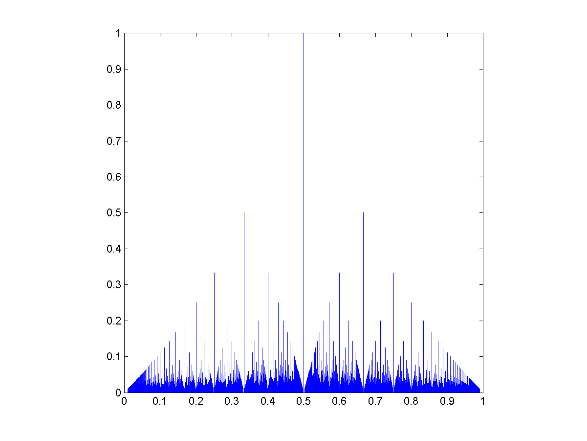
 where
where  :
:![The rational distribution of two convolved Exp[0.1] distributions.](http://aleph.se/andart2/wp-content/uploads/2014/09/trifonovexp01.png)
![Rational distribution of ratio between a Poisson[10] and a Poisson[5] variable.](http://aleph.se/andart2/wp-content/uploads/2014/09/trifonovpoiss105.png)