 During a recent party I got asked the question “Since
My first response was to point out that infinite decimal expressions are not enough: obviously 
If it is normal, then by the infinite monkey theorem then Shakespeare will almost surely be in the number. We actually do not know whether pi is normal, but it looks fairly likely. But that is not enough for a mathematician. A good overview of the problem can be found in a popular article by Bailey and Borwein. (Yep, one of the Borweins)
Where are the Shakespearian numbers?
This led to a second issue: what is the distribution of the Shakespeare-containing numbers?
We can encode Shakespeare in many ways. As an ASCII text the works take up 5.3 MB. One can treat this as a sequence of 7-bit characters and the works as 37,100,000 bits, or 11,168,212 decimal digits. A simple code where each pair of digits encode a character would encode 10,600,000 digits. This allows just a 100 character alphabet rather than a 127 character alphabet, but is likely OK for Shakespeare: we can use the ASCII code minus 32, for example.
If we denote the encoded works of Shakespeare by ![[Shakespeare]](https://s0.wp.com/latex.php?latex=%5BShakespeare%5D&bg=ffffff&fg=000000&s=0 "[Shakespeare]")
![0.[Shakespeare]xxxxx\ldots](https://s0.wp.com/latex.php?latex=0.%5BShakespeare%5Dxxxxx%5Cldots+&bg=ffffff&fg=000000&s=0 "0.[Shakespeare]xxxxx\ldots")
They form a rather tiny interval: since the works start with ‘The’, ![[0. 527269000\ldots , 0.52727]](https://s0.wp.com/latex.php?latex=%5B0.+527269000%5Cldots+%2C+0.52727%5D&bg=ffffff&fg=000000&s=0 "[0. 527269000\ldots , 0.52727]")
![[0,1]](https://s0.wp.com/latex.php?latex=%5B0%2C1%5D&bg=ffffff&fg=000000&s=0 "[0,1]")
But outside that interval there are numbers of the form ![0.y[Shakespeare]xxxx\ldots](https://s0.wp.com/latex.php?latex=0.y%5BShakespeare%5Dxxxx%5Cldots+&bg=ffffff&fg=000000&s=0 "0.y[Shakespeare]xxxx\ldots")


This pattern continues, with the intervals at each level ten times thinner but also 9 times as numerous. This is fairly similar to the Cantor set and gives rise to a fractal. But since the intervals are very tiny it is hard to see.
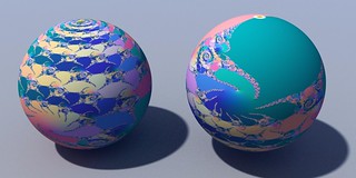
One way of visualizing this is to assume the weird encoding ![[Shakespeare]=3](https://s0.wp.com/latex.php?latex=%5BShakespeare%5D%3D3&bg=ffffff&fg=000000&s=0 "[Shakespeare]=3")
The fractal dimension of this Shakespeare-free set is /\log(10)\approx 0.9542")
In the case of the full 5.3MB [Shakespeare] the interval length is around 
/\log(10^{10,600,600}) \approx 1-\epsilon")

We have been looking at the unit interval. We can of course look at the entire real line too, but the pattern is similar: just magnify the unit interval pattern by 10, 100, 1000, … times. Somewhere around $10^{10,600,000}$ there are the numbers that have an integer part equal to ![[Shakespeare][Shakespeare]xxx\ldots](https://s0.wp.com/latex.php?latex=%5BShakespeare%5D%5BShakespeare%5Dxxx%5Cldots&bg=ffffff&fg=000000&s=0 "[Shakespeare][Shakespeare]xxx\ldots")
Shakespeare is common
One way of seeing that Shakespearian numbers are the generic case is to imagine choosing a number randomly. It has probability 
S+(9/10^2)S+\ldots = 10S<1")
Another way of thinking about it is just to look at the initial digits: the probability of starting with S")
S + (1-S)^2S + (1-S)^3S + \ldots = S/(1-(1-S))=1")
This might seem strange, since any number you are likely to mention is very likely Shakespeare-free. But this is just like the case of transcendental, normal or uncomputable numbers: they are actually the generic case in the reals, but most everyday numbers belong to the algebraic, non-normal and computable numbers.
It is also worth remembering that while all normal numbers are (almost surely) Shakespearian, there are non-normal Shakespearian numbers. For example, the fractional number ![0.[Shakespeare]000\ldots](https://s0.wp.com/latex.php?latex=0.%5BShakespeare%5D000%5Cldots+&bg=ffffff&fg=000000&s=0 "0.[Shakespeare]000\ldots")
![0.[Shakespeare][Shakespeare][Shakespeare]\ldots](https://s0.wp.com/latex.php?latex=0.%5BShakespeare%5D%5BShakespeare%5D%5BShakespeare%5D%5Cldots+&bg=ffffff&fg=000000&s=0 "0.[Shakespeare][Shakespeare][Shakespeare]\ldots")
![0.[Shakespeare]3141592\ldots](https://s0.wp.com/latex.php?latex=0.%5BShakespeare%5D3141592%5Cldots&bg=ffffff&fg=000000&s=0 "0.[Shakespeare]3141592\ldots")
In things of great receipt with case we prove,
Among a number one is reckoned none.
Then in the number let me pass untold,
Though in thy store’s account I one must be
-Sonnet 136
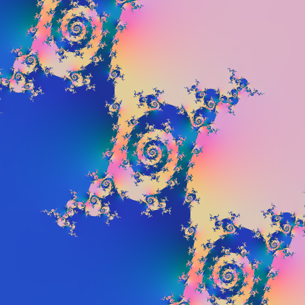
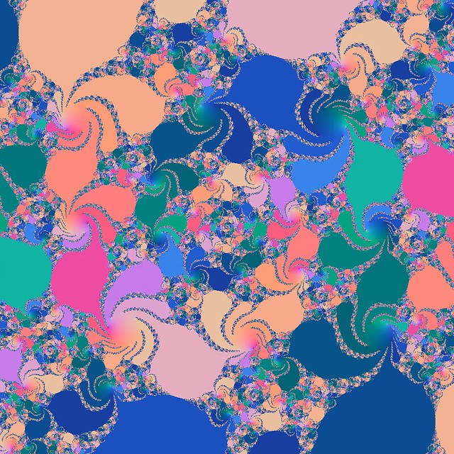
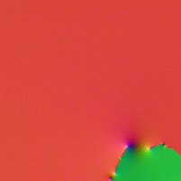
 = \tanh(cz_n)") , where c is a multiplicative constant. Iterating some number like 1 and plotting its fate produces the following “Mandelbrot set” in the c-plane – the colours here do not denote the time until escape to infinity but rather where in the complex plane the point ended up, as a function of c. In a normal Mandelbrot set infinity is an attractive fixed point; here it is just one place in the (extended) complex plane like any other.
, where c is a multiplicative constant. Iterating some number like 1 and plotting its fate produces the following “Mandelbrot set” in the c-plane – the colours here do not denote the time until escape to infinity but rather where in the complex plane the point ended up, as a function of c. In a normal Mandelbrot set infinity is an attractive fixed point; here it is just one place in the (extended) complex plane like any other.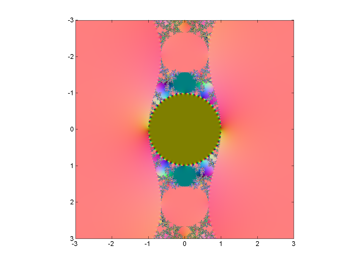
") . There is of course a corresponding negative solution since tanh is antisymmetric: if z is an attractive fixed point or cycle, so is -z. So the dynamics is always bistable.
. There is of course a corresponding negative solution since tanh is antisymmetric: if z is an attractive fixed point or cycle, so is -z. So the dynamics is always bistable.
 for integer
  . Since
 there are two real fixed points and a straight line border along the imaginary axis. This line of course contains the singularity points where things get sent to infinity, and near them the preimages of all the other singularities on the line: dramatic, but visually uninteresting.


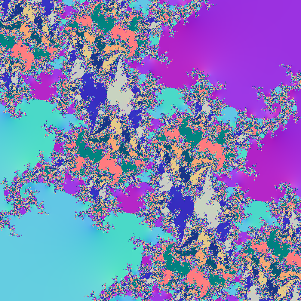

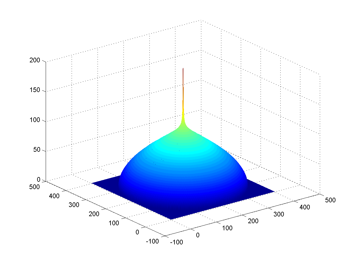
 we plot where iterates end up projected along some line (for example their real or imaginary part, or some combination). To make structure stand out a bit more I decided to color points after where in the whole plane they are, producing a colorful diagram for r=1.1:
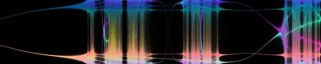
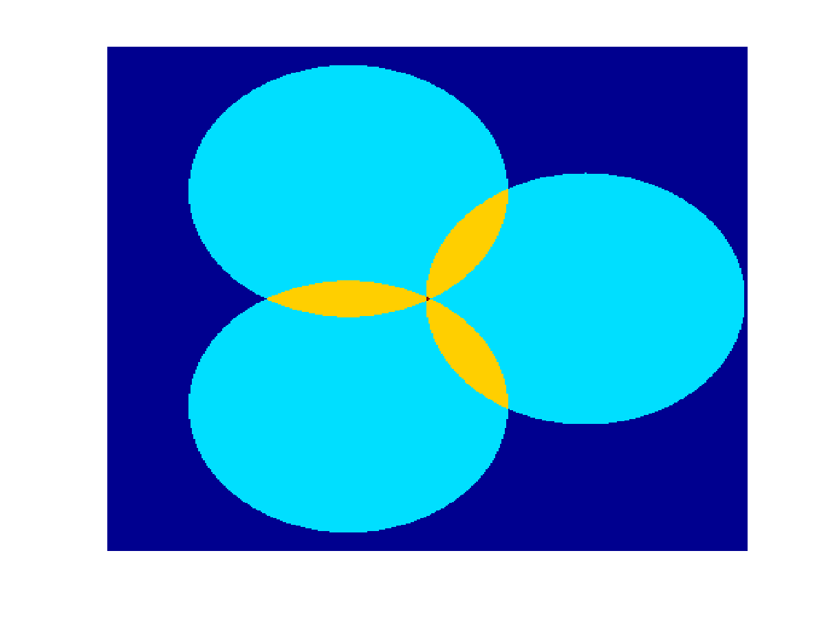
 is at the center, zero outside the borders.
 .
.
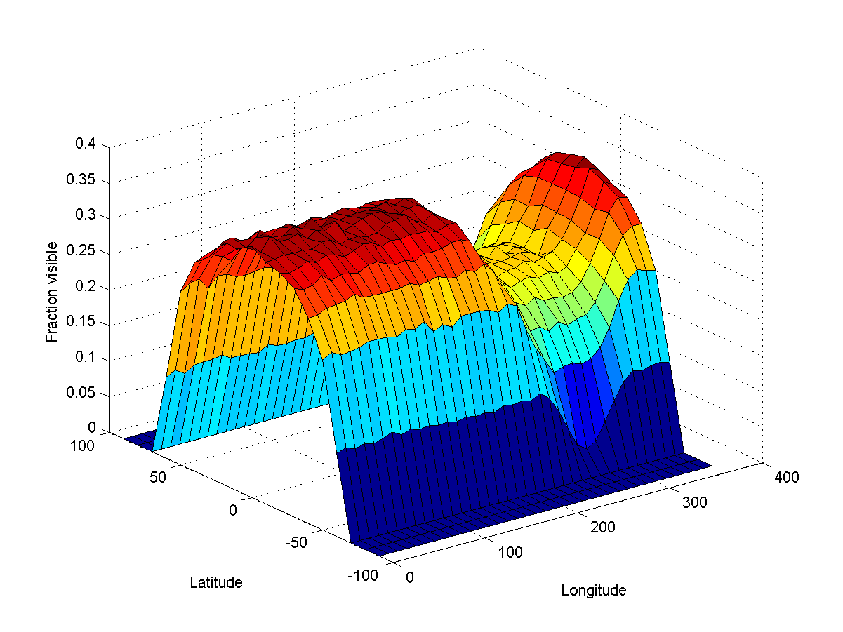
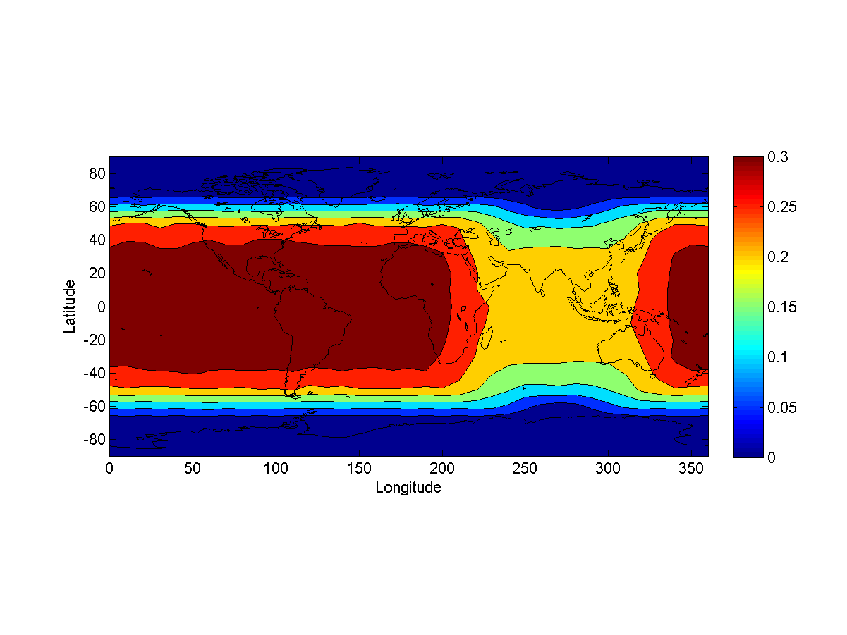
|\sin(\theta)|S") where
where  is the outer radius,
  the inner radius, $\theta$ the tilt (between 23 degrees for the summer/winter solstice and 0 for equinoxes) and
  for a New Years Eve firing, I get
  Watt.
Watt.

