What are the weirdest probability distributions I have encountered? Probably the fractal synaptic distribution.
There is no shortage of probability distributions: over any measurable space you can define some function that sums to 1, and you have a probability distribution. Since the underlying space can be integers, rational numbers, real numbers, complex numbers, vectors, tensors, computer programs, or whatever, and the set of functions tends to be big (the power set of the underlying space) there is a lot of stuff out there.
Lists of probability distributions involve a lot of named ones. But for every somewhat recognized distribution there are even more obscure ones.
In normal life I tend to encounter the usual distributions: uniform, Bernouilli, Beta, Gaussians, lognormal, exponential, Weibull (because of survival curves), Erlang (because of sums of exponentials), and a lot of power-laws because I am interested in extreme things.
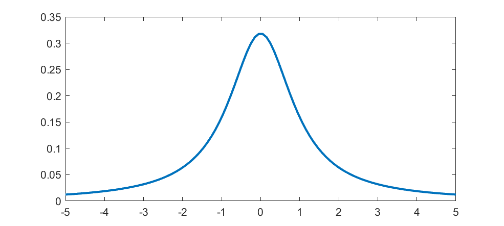 The first “weird” distribution I encountered was the Chauchy distribution. It has a nice algebraic form, a suggestive normalization constant… and no mean, variance or higher order moments. I remember being very surprised as a student when I saw that. It was there on the paper, with a very obvious centre point, yet that centre was not the mean. Like most “pathological examples” it was of course a representative of the majority: having a mean is actually quite “rare”. These days, playing with power-laws, I am used to this and indeed find it practically important. It is no longer weird.
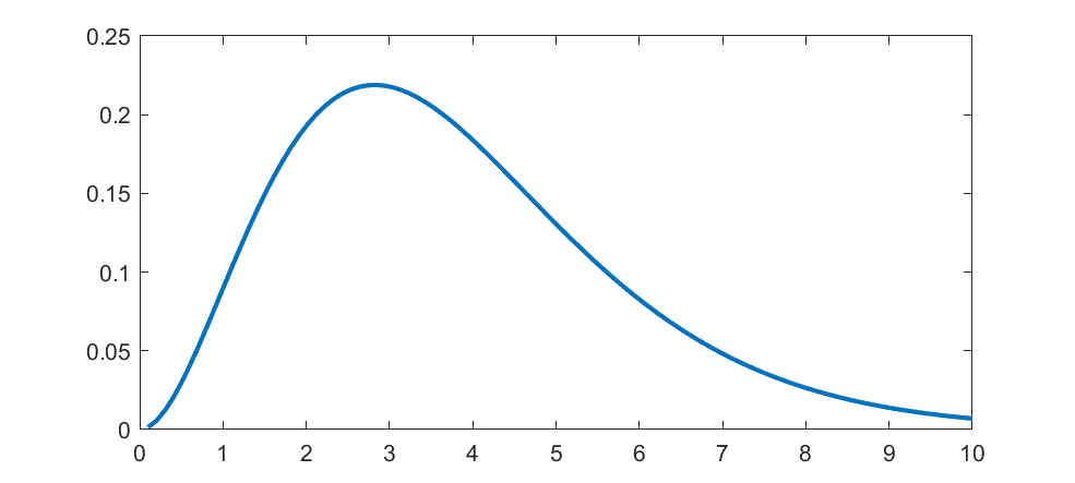 The Planck distribution isn’t too unusual, but has links to many cool special functions and is of course deeply important in physics. It is still surprisingly obscure as a mathematical probability distribution.
The weirdest distribution I have actually used (if only for a forgotten student report) is a fractal.
As a computational neuroscience student I looked into the distribution of synaptic weights in a forgetful attractor memory similar to the Hopfield network. In this case each weight would be updated with a +1 or -1 each time something was learned, added to the previous weight that had decayed somewhat: =k w(t) \pm 1, (0<k<1).")
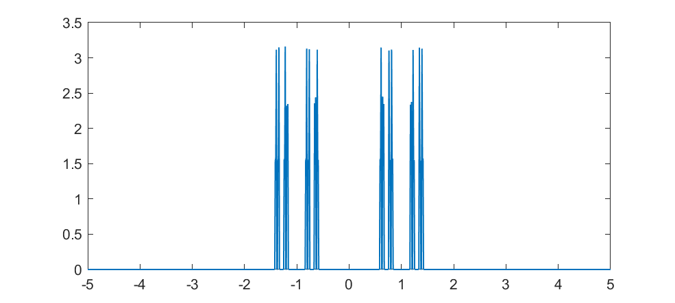
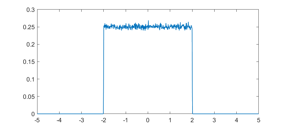
But what about intermediate cases? The update is basically mixing together two copies of the whole distribution. For small k, this produces a distribution across a Cantor set. As k increases the set gets thicker (that is, the fractal dimension increases towards 1), and at k=1/2 you get a uniform distribution. Indeed, it is a strange but true fact that you can not make a uniform distribution over the rational numbers in [0,1] but if we take an infinite sum obviously every single binary sequence will be possible and have equal probability, so it is the real number uniform distribution. Distributions and random numbers on the rationals are funny, since they are both discrete in the sense of being countable, yet so dense that most intuitions from discrete distributions fail and one tends to get fractal/recursive structures.
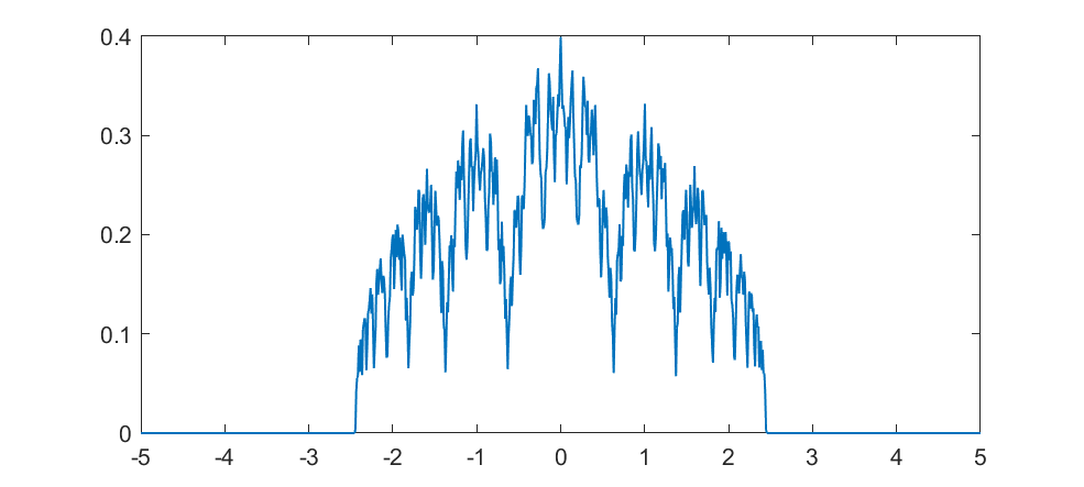
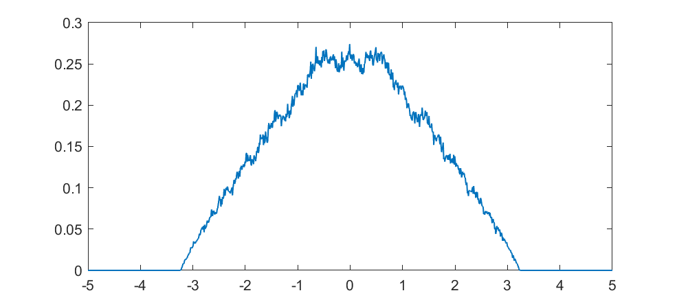
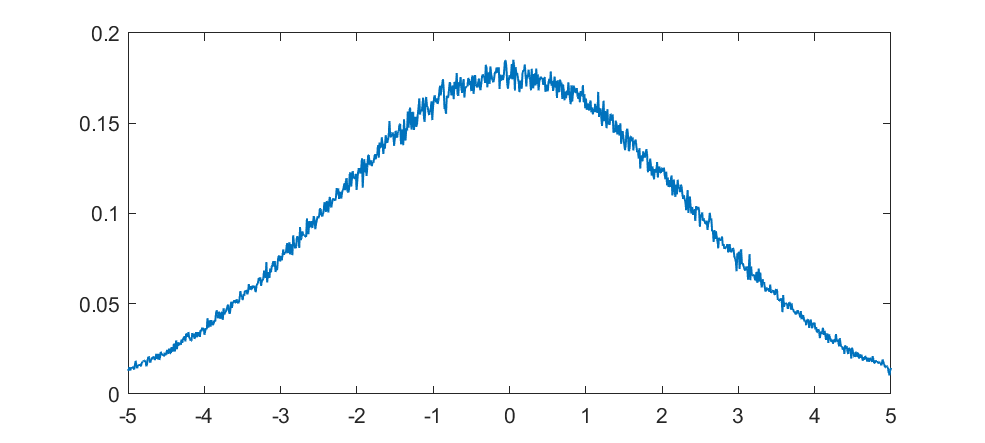
The real fun starts for k>1/2 since now peaks emerge on top of the uniform background. They happen because the two copies of the distribution blended together partially overlap, producing a recursive structure where there is a smaller peak between each pair of big peaks. This gets thicker and thicker, starting to look like a Weierstrass function curve and then eventually a Gaussian.
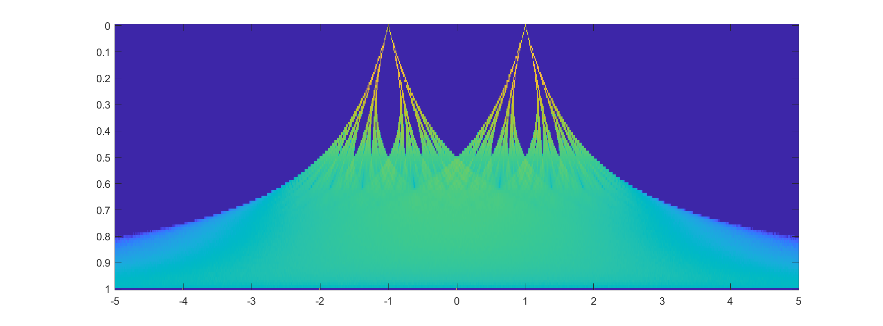
Plotting it in the (x,k) plane shows a neat overall structure, going from the Cantor sets to the fractal distributions towards the Gaussian (and, on the last k=1 row, the discrete Gaussian). The curves defining the edge of the distribution behave as ")
In practice, this distribution is unlikely to matter (real brains are too noisy and synapses do not work like that) but that doesn’t stop it from being neat.
 ). Then the ratio of the radii of the inner and outer circle will be
 )/(1+\sin(\pi/n))") . The radii of the circles in the ring will be
. The radii of the circles in the ring will be /2") and their centres are located at distance
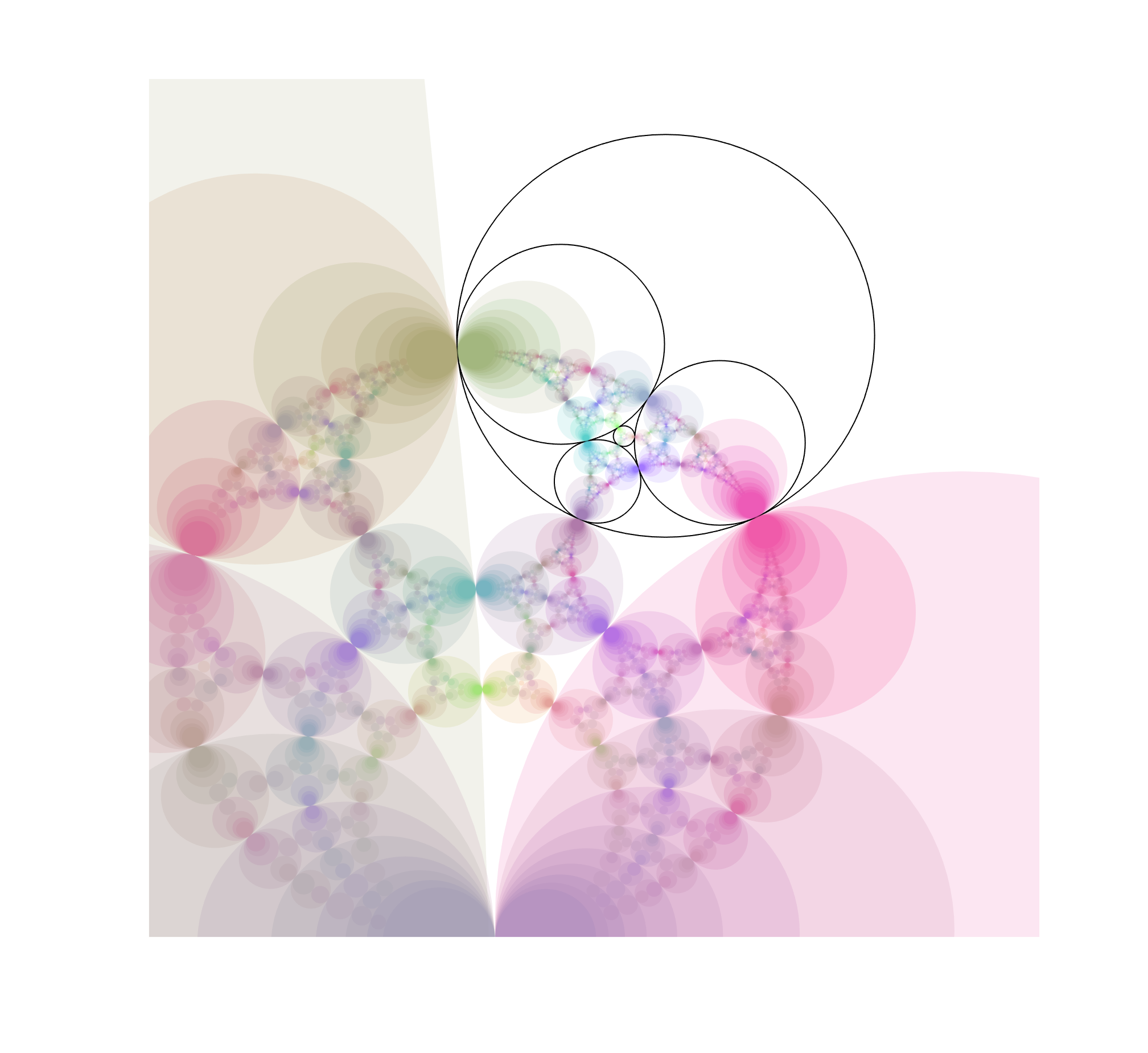
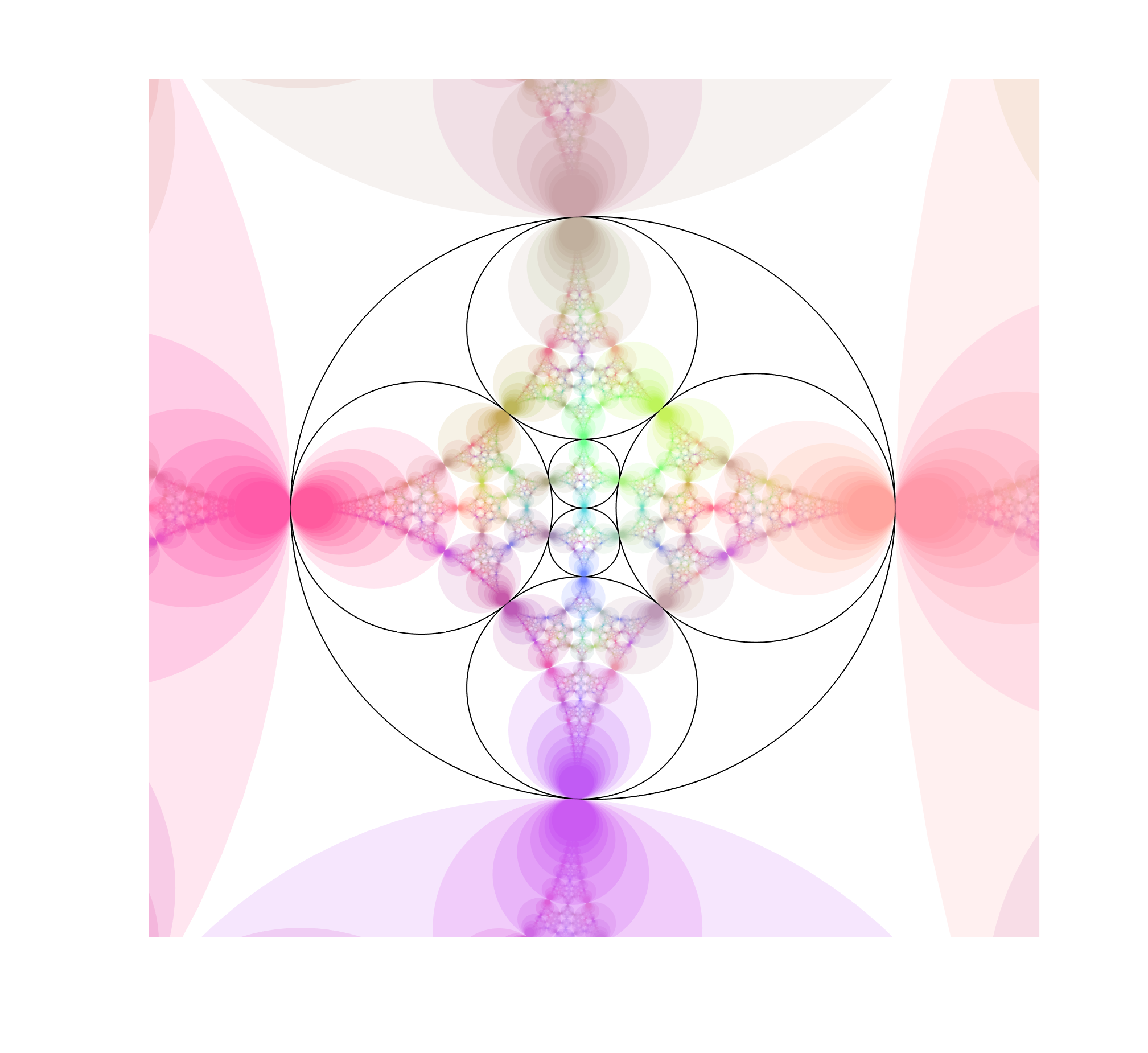
and their centres are located at distance /2") from the origin. This produces a staid concentric arrangement. Now invert with relation to an arbitrary circle: all the circles are mapped to other circles, their tangencies preserved. Voila! A suitably eccentric Steiner chain to play with.
from the origin. This produces a staid concentric arrangement. Now invert with relation to an arbitrary circle: all the circles are mapped to other circles, their tangencies preserved. Voila! A suitably eccentric Steiner chain to play with. and radius
  the map
 =(w+z)r") maps the interior of the unit circle to it. Use the ease of rotating the original concentric ring to produce an animation, and we can reconstruct the fractal.
maps the interior of the unit circle to it. Use the ease of rotating the original concentric ring to produce an animation, and we can reconstruct the fractal.


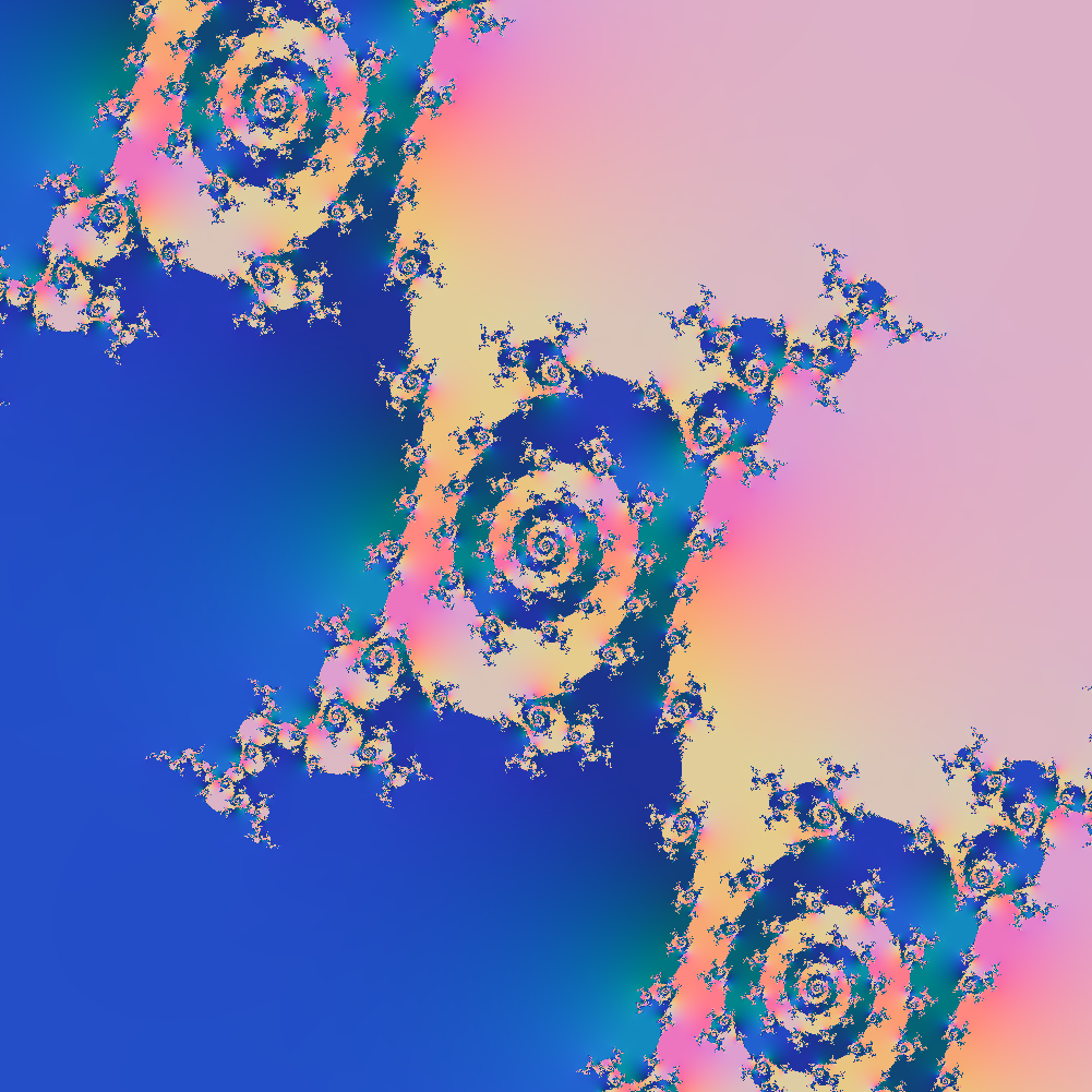
 = \tanh(cz_n)") , where c is a multiplicative constant. Iterating some number like 1 and plotting its fate produces the following “Mandelbrot set” in the c-plane – the colours here do not denote the time until escape to infinity but rather where in the complex plane the point ended up, as a function of c. In a normal Mandelbrot set infinity is an attractive fixed point; here it is just one place in the (extended) complex plane like any other.
, where c is a multiplicative constant. Iterating some number like 1 and plotting its fate produces the following “Mandelbrot set” in the c-plane – the colours here do not denote the time until escape to infinity but rather where in the complex plane the point ended up, as a function of c. In a normal Mandelbrot set infinity is an attractive fixed point; here it is just one place in the (extended) complex plane like any other.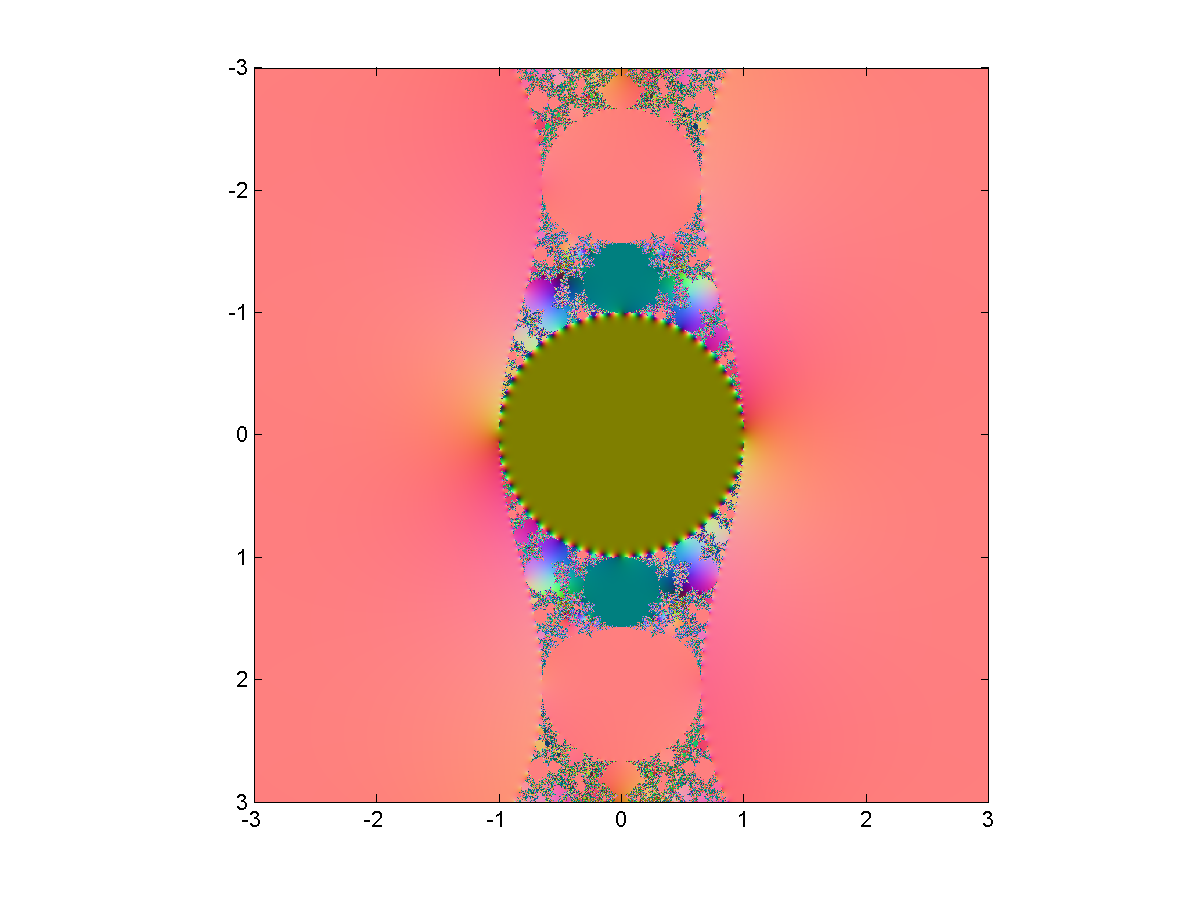
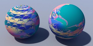
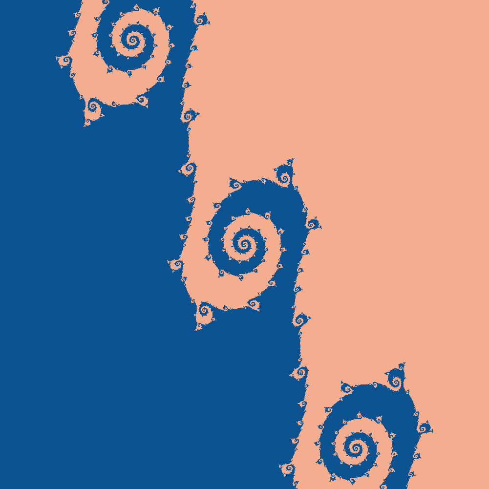
") . There is of course a corresponding negative solution since tanh is antisymmetric: if z is an attractive fixed point or cycle, so is -z. So the dynamics is always bistable.
. There is of course a corresponding negative solution since tanh is antisymmetric: if z is an attractive fixed point or cycle, so is -z. So the dynamics is always bistable.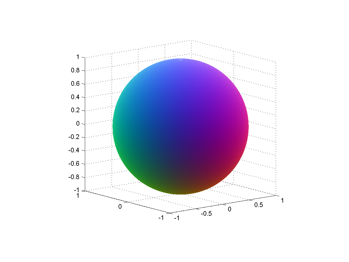
 for integer
  . Since
 there are two real fixed points and a straight line border along the imaginary axis. This line of course contains the singularity points where things get sent to infinity, and near them the preimages of all the other singularities on the line: dramatic, but visually uninteresting.
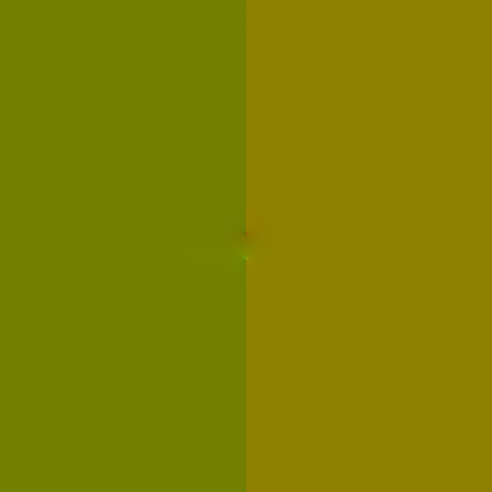


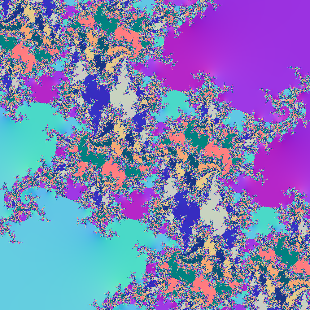

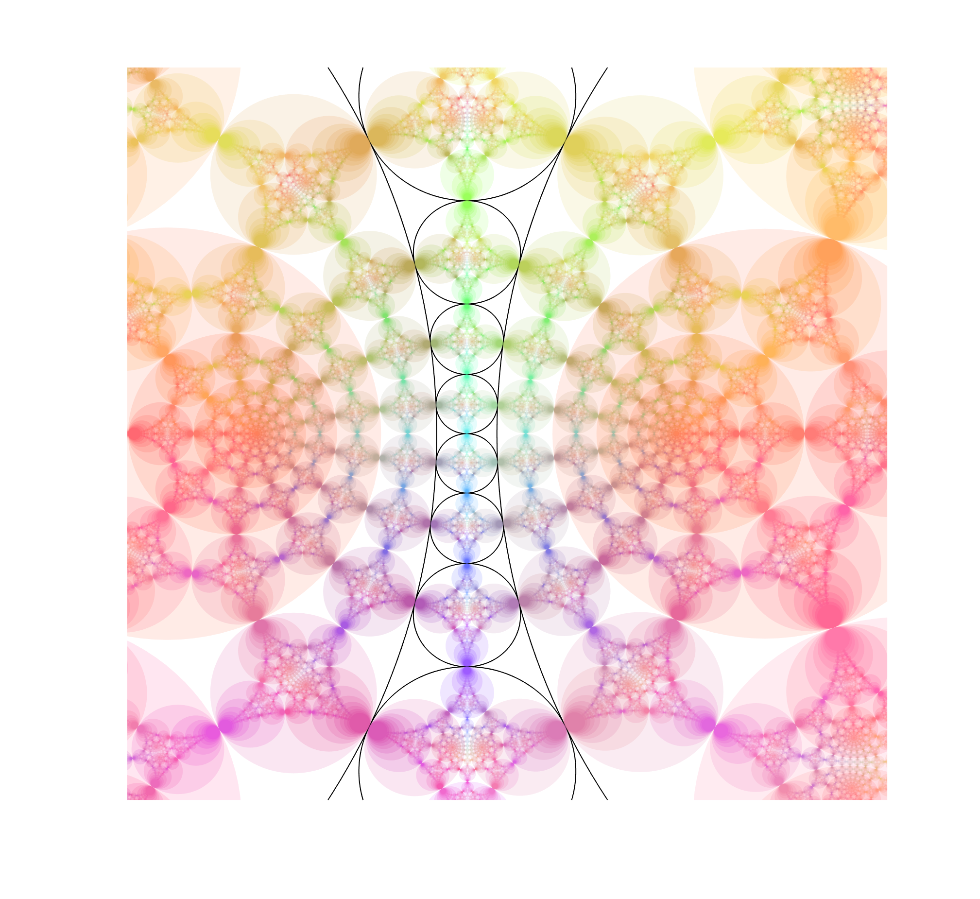
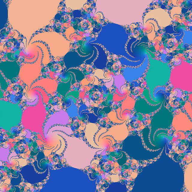
 we plot where iterates end up projected along some line (for example their real or imaginary part, or some combination). To make structure stand out a bit more I decided to color points after where in the whole plane they are, producing a colorful diagram for r=1.1:
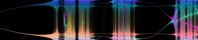
 is at the center, zero outside the borders.
 .
.