What about nested/continued integrals? Here is a simple one:
.
The way to see this is to recognize that the x in the first integral is going to integrate to , the x in the second will be integrated twice , and so on.
In general additive integrals of this kind turn into sums (assuming convergence, handwave, handwave…):
.
On the other hand, .
So if we insert we get the sum . For we end up with . The differential equation has solution . Setting the integral is clearly zero, so . Tying it together we get:
.
Things are trickier when the integrals are multiplicative, like . However, we can turn it into a differential equation: which has the well known solution . Same thing for , giving us . Since we are running indefinite integrals we get those pesky constants.
Plugging in gives . If we set we get the mildly amusing and in retrospect obvious formula
.
We can of course mess things up further, like , where the differential equation becomes with the solution . A surprisingly simple solution to a weird-looking integral. In a similar vein:
(that is, you get an implicit but well defined expression for the (x,I(x)) values. With Lambert, the x and y axes always tend to switch place).
[And yes, convergence is handwavy in this essay. I think the best way of approaching it is to view the values of these integrals as the functions invariant under the functional consisting of the integral and its repeated function: whether nearby functions are attracted to it (or not) under repeated application of the functional depends on the case. ]
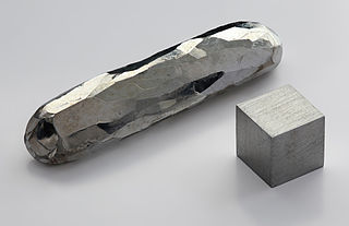
Background: in WW2, Heisenberg was working on the German atomic reactor project (was he bad? see the fascinating play “Copenhagen” to find out!). His team almost finished a nuclear reactor. He thought that a reaction with natural uranium would be self-limiting (spoiler: it wouldn’t), so had no cadmium control rods or other means of stopping a chain reaction.
But, no worries: his team has “a lump of cadmium” that they could toss into the reactor if things got out of hand. So, now, if someone has a level of precaution woefully inadequate to the risk at hand, I will call it a lump of cadmium.
To understand it we must say something about Heisenberg’s concept of reactor design. He persuaded himself that a reactor designed with natural uranium and, say, a heavy water moderator would be self-stabilizing and could not run away. He noted that U(238) has absorption resonances in the 1-eV region, which means that a neutron with this kind of energy has a good chance of being absorbed and thus removed from the chain reaction. This is one of the challenges in reactor design—slowing the neutrons with the moderator without losing them all to absorption. Conversely, if the reactor begins to run away (become supercritical) , these resonances would broaden and neutrons would be more readily absorbed. Moreover, the expanding material would lengthen the mean free paths by decreasing the density and this expansion would also stop the chain reaction. In short, we might experience a nasty chemical explosion but not a nuclear holocaust. Whether Heisenberg realized the consequences of such a chemical explosion is not clear. In any event, no safety elements like cadmium rods were built into Heisenberg’s reactors. At best, a lump of cadmium was kepton hand in case things threatened to get out of control. He also never considered delayed neutrons, which, as we know, play an essential role in reactor safety. Because none of Heisenberg’s reactors went critical, this dubious strategy was never put to the test.
(Jeremy Bernstein, Heisenberg and the critical mass. Am. J. Phys. 70, 911 (2002); http://dx.doi.org/10.1119/1.1495409)
This reminds me a lot of the modelling errors we discuss in the “Probing the improbable” paper, especially of course the (ahem) energetic error giving Castle Bravo 15 megatons of yield instead of the predicted 4-8 megatons. Leaving out Li(7) from the calculations turned out to leave out the major contributor of energy.
Note that Heisenberg did have an argument for his safety, in fact two independent ones! The problem might have been that he was thinking in terms of mostly U(238) and then getting any kind of chain reaction going would be hard, so he was biased against the model of explosive chain reactions (but as the Bernstein paper notes, somebody in the project had correct calculations for explosive critical masses). Both arguments were flawed when dealing with reactors enriched in U(235). Coming at nuclear power from the perspective of nuclear explosions on the other hand makes it natural to consider how to keep things from blowing up.
We may hence end up with lumps of cadmium because we approach a risk from the wrong perspective. The antidote should always be to consider the risks from multiple angles, ideally a few adversarial ones. The more energy, speed or transformative power we expect something to produce, the more we should scrutinize existing safeguards for them being lumps of cadmium. If we think our project does not have that kind of power, we should both question why we are even doing it, and whether it might actually have some hidden critical mass.
And, yes, the use of “infinite impact” grates on me – it must be interepreted as “so bad that it is never acceptable”, a ruin probability, or something similar, not that the disvalue diverges. But the overall report is a great start on comparing and analysing the big risks. It is worth comparing it with the WEF global risk report, which focuses on people’s perceptions of risk. This one aims at looking at what risks are most likely/impactful. Both try to give reasons and ideas for how to reduce the risks. Hopefully they will also motivate others to make even sharper analysis – this is a first sketch of the domain, rather than a perfect roadmap. Given the importance of the issues, it is a bit worrying that it has taken us this long.
The gamma function has a long and interesting history (check out (Davis 1963) excellent review), but one application does not seem to have shown up: minimal surfaces.
A minimal surface is one where the average curvature is always zero; it bends equally in two opposite directions. This is equivalent to having the (locally) minimal area given its boundary: such surfaces are commonly seen as soap films stretched from frames. There exists a rich theory for them, linking them to complex analysis through the Enneper-Weierstrass representation: if you have a meromorphic function g and an analytic function f such that is holomorphic, then
produces a minimal surface .
When plugging in the hyperbolic tangent as g and using f=1 I got a new and rather nifty surface a few years back. What about plugging in the gamma function? Let .
We integrate from the regular point to different points in the complex plane. Let us start with the simple case of .
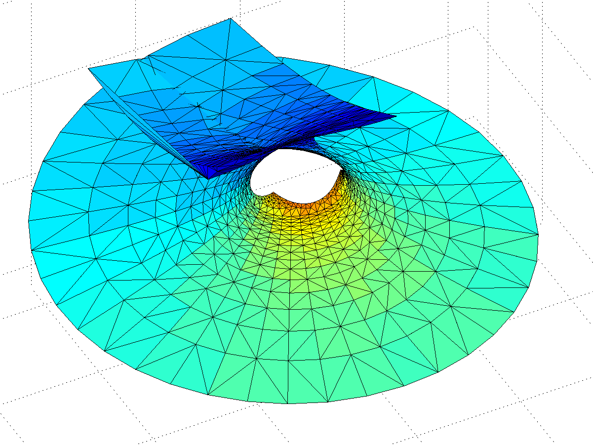
Gamma function minimal surface for z in 0.5<Re(z)<3.5, -8<Im(z)
The surface is a billowing strip, and as we include z with larger and larger real parts the amplitude of the oscillations grow rapidly, making it self-intersect. The behaviour is somewhat similar to the Catalan minimal surface, except that we only get one period. If we go to larger imaginary parts the surface approaches a horizontal plane. OK, the surface is a plane with some wild waves, right?
Not so fast, we have not looked at the mess for Re(z)<0. First, let’s examine the area around the z=0 singularity. Since the values of the integrand blows up close to it, they produce a surface expanding towards infinity – very similar to a catenoid. Indeed, catenoid ends tend to show up where there are poles. But this one doesn’t close exactly: for re(z)<0 there is some overshoot producing a self-intersecting plane-like strip.
Gamma function minimal surface close to the z=0 singularity. Colour denotes Re(z). Integration contours from 1 to z run clockwise for Im(z)<0 and counterclockwise for Im(z)>0.
The problem is of course the singularity: when integrating in the complex plane we need to avoid them, and depending on the direction we go around them we can get a complex phase that gives us an entirely different value of the function. In this case the branch cut corresponds to the real line: integrating clockwise or counter-clockwise around z=0 to the same z gives different values. In fact, a clockwise turn adds [3.6268i, 3.6268, 6.2832i] (which looks like – a rather neat residue!) to the coordinates: a translation in the positive y-direction. If we extend the surface by going an extra turn clockwise or counterclockwise a number of times, we get copies that attach seamlessly.
Gamma minimal surface extended by integration paths between the -1 and 0 singularities (blue patches).
Gamma minimal surface patch that can be repeated by translation along the y-axis. Colour denotes Re(z).
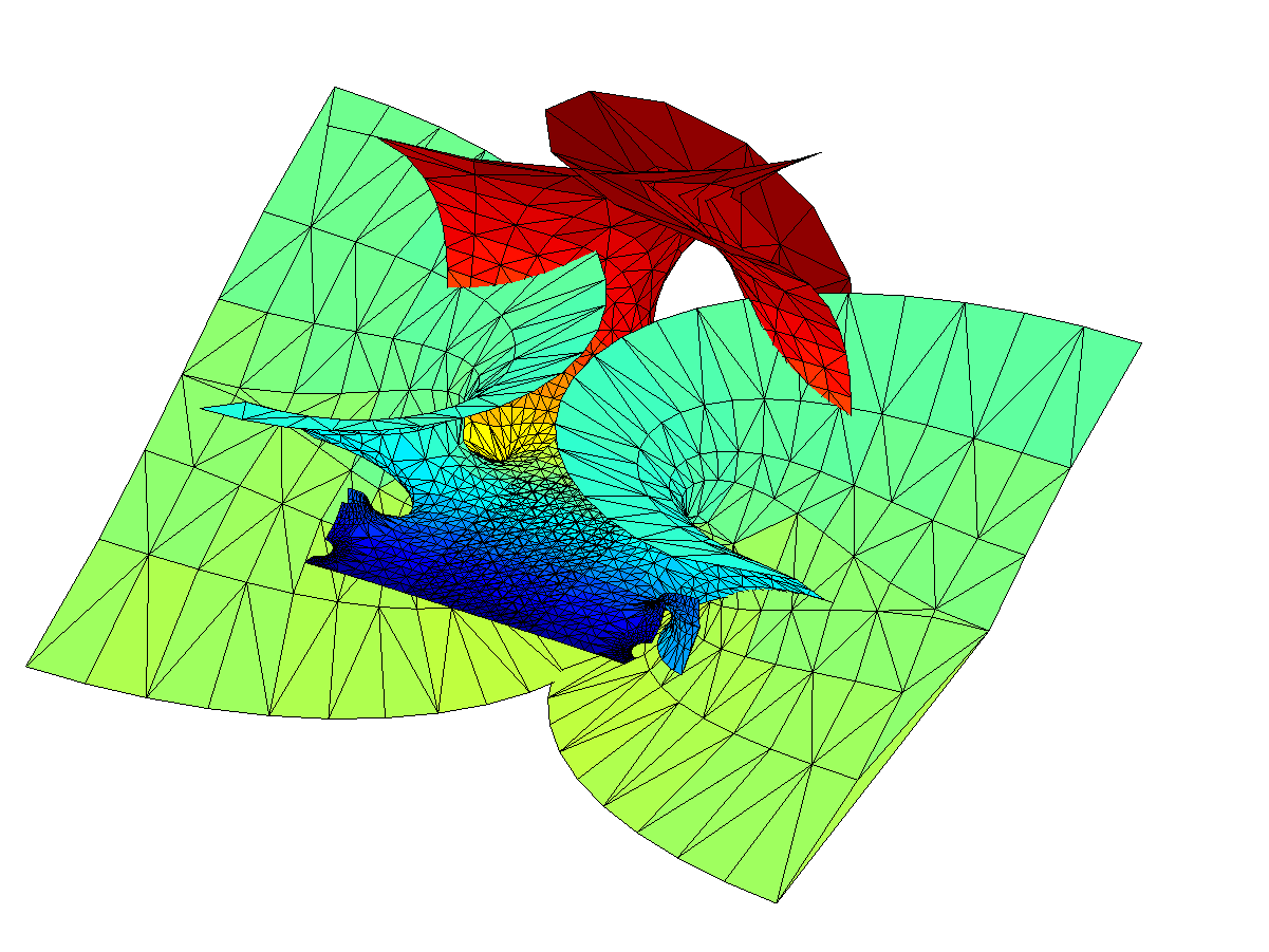
OK, we have a surface with some planar strips that turn wobbly and self-intersecting in the x-direction, with elliptic catenoid ends repeating along the y-direction due to the z=0 singularity. Going down the negative x-direction things look plane between the catenoids… except of course for the catenoids due to all the other singularities for . They also introduce residues along the y-direction, but different ones from the z=0 – their extensions of the surface will be out of phase with each other, making the fully extended surface fantastically self-intersecting and confusing.
Gamma function minimal surface extended by integrating around poles.
So, I think we have a simple answer to why the gamma function minimal surface is not well known: it is simply too messy and self-intersecting.
Of course, there may be related nifty surfaces. is nicely behaved and looks very much like the Enneper surface near zero, with “wings” that oscillate ever more wildly as we move towards the negative reals. No doubt there are other beautiful things to look for in the vicinity.
There are some texts that are worth reading, even if you are outside the group they are intended for. Here is one that I think everybody should read at least the first half of:
Haldane, the Executive Director for Financial Stability at Bank of England, brings up the topic is how to act in situations of uncertainty, and the role of our models of reality in making the right decision. How complex should they be in the face of a complex reality? The answer, based on the literature on heuristics, biases and modelling, and the practical world of financial disasters, is simple: they should be simple.
Using too complex models means that they tend to overfit scarce data, weight data randomly, require significant effort to set up – and tends to promote overconfidence. As Haldane then moves on to his own main topic, banking regulation. Complex regulations – which are in a sense models of how banks ought to act – have the same problem, and also act as incentives for playing the rules to gain advantage. The end result is an enormous waste of everybody’s time and effort that does not give the desired reduction of banking risk.
It is striking how many people have been seduced by the siren call of complex regulation or models, thinking their ability to include every conceivable special case is a sign of strength. Finance and finance regulation are full of smart people who make the same mistake, as is science. If there is one thing I learned in computational biology is that your model better produce more nontrivial results than the number of parameters it has.
But coming up with simple rules or models is not easy: knowing what to include and what not to include requires expertise and effort. In many ways this may be why people like complex models, since there are no tricky judgement calls.
Another of my favourite functions if the Gamma function, , the continuous generalization of the factorial. While it grows rapidly for positive reals, it has fun poles for the negative integers and is generally complex. What happens when you iterate it?
First I started by just applying it to different starting points, . The result is a nice fractal, with some domains approaching 1, and others running off to infinity.
Here I color points that go to infinity in green shades on the number of iterations before they become very large, and the points approaching 1 by . Zooming in a bit more reveals neat self-similar patterns with alternating “beans”:
In the outside regions we have thin tendrils stretching towards infinity. These are familiar to anybody who has been iterating exponentials or trigonometric functions: the combination of oscillation and (super)exponential growth leads to the pattern.
OK,that was a Julia set (different starting points, same formula). What about a counterpart to the Mandelbrot set? I looked at where c is the control parameter. I start with and iterate:
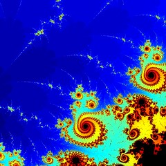
Zooming in shows the same kind of motif copies of Julia sets as we see in the quadratic Mandelbrot set:
In fact, zooming in as above in the counterpart to the “seahorse valley” shows a remarkable similarity.
After a recent lecture about the singularity I got asked about its energy requirements. It is a good question. As my inquirer pointed out, humanity uses more and more energy and it generally has an environmental cost. If it keeps on growing exponentially, something has to give. And if there is a real singularity, how do you handle infinite energy demands?
First I will look at current trends, then different models of the singularity.
I will not deal directly with environmental costs here. They are relative to some idea of a value of an environment, and there are many ways to approach that question.
Current trends
Current computers are energy hogs. Currently general purpose computing consumes about one Petawatt-hour per year, with the entire world production somewhere above 22 Pwh. While large data centres may be obvious, the vast number of low-power devices may be an even more significant factor; up to 10% of our electricity use may be due to ICT.
Koomey’s law states that the number of computations per joule of energy dissipated has been doubling approximately every 1.57 years. This might speed up as the pressure to make efficient computing for wearable devices and large data centres makes itself felt. Indeed, these days performance per watt is often more important than performance per dollar.
Semilog plot of global energy (all types) consumption over time.
Looking at overall energy use trends it looks like overall energy use increases exponentially (but has stayed at roughly the same per capita level since the 1970s). In fact, plotting it on a semilog graph suggests that it is increasing faster than exponential (otherwise it would be a straight line). This is presumably due to a combination of population increase and increased energy use. The best fit exponential has a doubling time of 44.8 years.
Electricity use is also roughly exponential, with a doubling time of 19.3 years. So we might be shifting more and more to electricity, and computing might be taking over more and more of that.
Extrapolating wildly, we would need the total solar input on Earth in about 300 years and the total solar luminosity in 911 years. In about 1,613 years we would have used up the solar system’s mass energy. So, clearly, long before then these trends will break one way or another.
Physics places a firm boundary due to the Landauer principle: in order to erase on bit of information joules of energy have to be dissipated. Given current efficiency trends we will reach this limit around 2048.
The principle can be circumvented using reversible computation, either classical or quantum. But as I often like to point out, it still bites in the form of the need for error correction (erasing accidentally flipped bits) and formatting new computational resources (besides the work in turning raw materials into bits). We should hence expect a radical change in computation within a few decades, even if the cost per computation and second continues to fall exponentially.
What kind of singularity?
But how many joules of energy does a technological singularity actually need? It depends on what kind of singularity. In my own list of singularity meanings we have the following kinds:
A. Accelerating change
B. Self improving technology
C. Intelligence explosion
D. Emergence of superintelligence
E. Prediction horizon
F. Phase transition
G. Complexity disaster
H. Inflexion point
I. Infinite progress
Case A, acceleration, at first seems to imply increasing energy demands, but if efficiency grows faster they could of course go down.
He suggests energy rate density may increase as Moore’s law, at least in our current technological setting. If we assume this to be true, then we would have , where is the power of the system and is the mass of the system at time t. One can maintain exponential growth by reducing the mass as well as increasing the power.
However, waste heat will need to be dissipated. If we use the simplest model where a radius R system with density radiates it away into space, then the temperature will be , or, if we have a maximal acceptable temperature, . So the system needs to become smaller as increases. If we use active heat transport instead (as outlined in my previous post), covering the surface with heat pipes that can remove X watts/square meter, then . Again, the radius will be inversely proportional to . This is similar to our current computers, where the CPU is a tiny part surrounded by cooling and energy supply.
If we assume the waste heat is just due to erasing bits, the rate of computation will be bits per second. Using the first cooling model gives us – a massive advantage for running extremely hot and dense computation. In the second cooling model : in both cases higher energy rate densities make it harder to compute when close to the thermodynamic limit. Hence there might be an upper limit to how much we may want to push .
Also, a system with mass M will use up its own mass-energy in time : the higher the rate, the faster it will run out (and it is independent of size!). If the system is expanding at speed v it will gain and use up mass at a rate ; if grows faster than quadratic with time it will eventually run out of mass to use. Hence the exponential growth must eventually reduce simply because of the finite lightspeed.
The Chaisson scenario does not suggest a “sustainable” singularity. Rather, it suggests a local intense transformation involving small, dense nuclei using up local resources. However, such local “detonations” may then spread, depending on the long-term goals of involved entities.
Cases B, C, D(intelligence explosions, superintelligence) have an unclear energy profile. We do not know how complex code would become or what kind of computational search is needed to get to superintelligence. It could be that it is more a matter of smart insights, in which case the needs are modest, or a huge deep learning-like project involving massive amounts of data sloshing around, requiring a lot of energy.
Case E, a prediction horizon, is separate from energy use. As this essay shows, there are some things we can say about superintelligent computational systems based on known physics that likely remains valid no matter what.
Case F, phase transition, involves a change in organisation rather than computation, for example the formation of a global brain out of previously uncoordinated people. However, this might very well have energy implications. Physical phase transitions involve discontinuities of the derivatives of the free energy. If the phases have different entropies (first order transitions) there has to be some addition or release of energy. So it might actually be possible that a societal phase transition requires a fixed (and possibly large) amount of energy to reorganize everything into the new order.
There are also second order transitions. These are continuous do not have a latent heat, but show divergent susceptibilities (how much the system responds to an external forcing). These might be more like how we normally imagine an ordering process, with local fluctuations near the critical point leading to large and eventually dominant changes in how things are ordered. It is not clear to me that this kind of singularity would have any particular energy requirement.
Case G, complexity disaster, is related to superexponential growth, such as the city growth model of Bettancourt, West et al. or the work on bubbles and finite time singularities by Didier Sornette. Here the rapid growth rate leads to a crisis, or more accurately a series of crises increasingly rapidly succeeding each other until a final singularity. Beyond that the system must behave in some different manner. These models typically predict rapidly increasing resource use (indeed, this is the cause of the crisis sequence as one kind of growth runs into resource scaling problems and is replaced with another one), although as Sornette points out the post-singularity state might well be a stable non-rivalrous knowledge economy.
Case H, an inflexion point, is very vanilla. It would represent the point where our civilization is halfway from where we started to where we are going. It might correspond to “peak energy” where we shift from increasing usage to decreasing usage (for whatever reason), but it does not have to. It could just be that we figure out most physics and AI in the next decades, become a spacefaring posthuman civilization, and expand for the next few billion years, using ever more energy but not having the same intense rate of knowledge growth as during the brief early era when we went from hunter gatherers to posthumans.
Case I, infinite growth, is not normally possible in the physical universe. Information can as far as we know not be stored beyond densities set by the Bekenstein bound ( where bits per kg per meter), and we only have access to a volume with mass density , so the total information growth must be bounded by . It grows quickly, but still just polynomially.
The exception to the finitude of growth is if we approach the boundaries of spacetime. Frank J. Tipler’s omega point theory shows how information processing could go infinite in a finite (proper) time in the right kind of collapsing universe with the right kind of physics. It doesn’t look like we live in one, but the possibility is tantalizing: could we arrange the right kind of extreme spacetime collapse to get the right kind of boundary for a mini-omega? It would be way beyond black hole computing and never be able to send back information, but still allow infinite experience. Most likely we are stuck in finitude, but it won’t hurt poking at the limits.
Conclusions
Indefinite exponential growth is never possible for physical properties that have some resource limitation, whether energy, space or heat dissipation. Sooner or later they will have to shift to a slower rate of growth – polynomial for expanding organisational processes (forced to this by the dimensionality of space, finite lightspeed and heat dissipation), and declining growth rate for processes dependent on a non-renewable resource.
That does not tell us much about the energy demands of a technological singularity. We can conclude that it cannot be infinite. It might be high enough that we bump into the resource, thermal and computational limits, which may be what actually defines the singularity energy and time scale. Technological singularities may also be small, intense and localized detonations that merely use up local resources, possibly spreading and repeating. But it could also turn out that advanced thinking is very low-energy (reversible or quantum) or requires merely manipulation of high level symbols, leading to a quiet singularity.
My own guess is that life and intelligence will always expand to fill whatever niche is available, and use the available resources as intensively as possible. That leads to instabilities and depletion, but also expansion. I think we are – if we are lucky and wise – set for a global conversion of the non-living universe into life, intelligence and complexity, a vast phase transition of matter and energy where we are part of the nucleating agent. It might not be sustainable over cosmological timescales, but neither is our universe itself. I’d rather see the stars and planets filled with new and experiencing things than continue a slow dance into the twilight of entropy.
…contemplate the marvel that is existence and rejoice that you are able to do so. I feel I have the right to tell you this because, as I am inscribing these words, I am doing the same. – Ted Chiang, Exhalation
The ever awesome Scott Alexander made a map of the rationalist blogosphere (webosphere? infosphere?) that I just saw (hat tip to Waldemar Ingdahl). Besides having plenty of delightful xkcd-style in-jokes, it is also useful by showing me parts of my intellectual neighbourhood I did not know well and might want to follow (want to follow, but probably can’t follow because of time constraints).
He starts out with pointing at some other concept maps like that, both the classic xkcd one and Julia Galef’s map of Bay Area memespace, which was a pleasant surprise to me. The latter explains the causal/influence links between communities in a very clear way.
One can of course quibble endlessly on what is left in or out (I loved the comments about the apparent lack of dragons on the rationalist map), but the two maps also show two different approaches to relatedness. In the rationalist map distance is based on some form of high-dimensional similarity, crunching it down to 2D using an informal version of a Kohonen map. Bodies of water can be used to “cheat” and add discontinuities/tears. In the memespace map the world is a network of causal/influence links, and the overall similarities between linked groups can be slight even when they share core memes. Here the cheating consists of leaving out broad links (Burning Man is mentioned; it would connect many nodes weakly to each other). In both cases what is left out is important, just as the choice of resolution. Good maps show the information the creator wants to show, and communicates it well.


dx\right)dx\right)dx")


=\int f(x)+\left(\int f(x)+\left(\int f(x)+\left(\ldots\right)dx\right)dx\right)dx = \sum_{n=1}^\infty \int^n f(x) dx")
=f(x)+I(x)")
=\sin(kx)")
=-\cos(kx)/k-\sin(kx)/k^2+\cos(kx)/k^3+\sin(x)/k^4-\cos(kx)/k^5-\ldots")

=\sum_{n=0}^\infty 1/k^{4n+2} - \sum_{n=0}^\infty 2/k^{4n+1}")
=ce^x-\sin(kx)/(k^2+1) - k\cos(kx)/(k^2+1)")


")
=\int x \int x \int x \ldots dx dx dx")
=x I(x)")
=ce^{x^2/2}")
=ce^{-\cos(kx)/k}")
=1/x")
=cx")


=\int\sqrt{\int\sqrt{\int\sqrt{\ldots} dx} dx} dx")

=(1/4)(c^2 + 2cx + x^2)")
=\int\sin\left(\int\sin\left(\int\sin\left(\ldots\right)dx\right) dx\right) dx")
=\int \exp\left(\int \exp\left(\int \exp\left(\ldots \right) dx \right) dx \right) dx")
=\int \left(\int \left(\int \left(\ldots \right)^2 dx \right)^2 dx \right)^2 dx")
=\int W\left(\int W\left(\int W\left(\ldots \right) dx \right) dx \right) dx")
}1/W(t) dt + c")

 is holomorphic, then
=\Re\left(\int_{z_0}^z f(1-g^2)/2 dz\right)")
=\Re\left(\int_{z_0}^z if(1+g^2)/2 dz\right)")
=\Re\left(\int_{z_0}^z fg dz\right)")
,Y(z),Z(z))") .
.") .
. to different points
  in the complex plane. Let us start with the simple case of
 >1/2") .
.
 – a rather neat residue!) to the coordinates: a translation in the positive y-direction. If we extend the surface by going an extra turn clockwise or counterclockwise a number of times, we get copies that attach seamlessly.
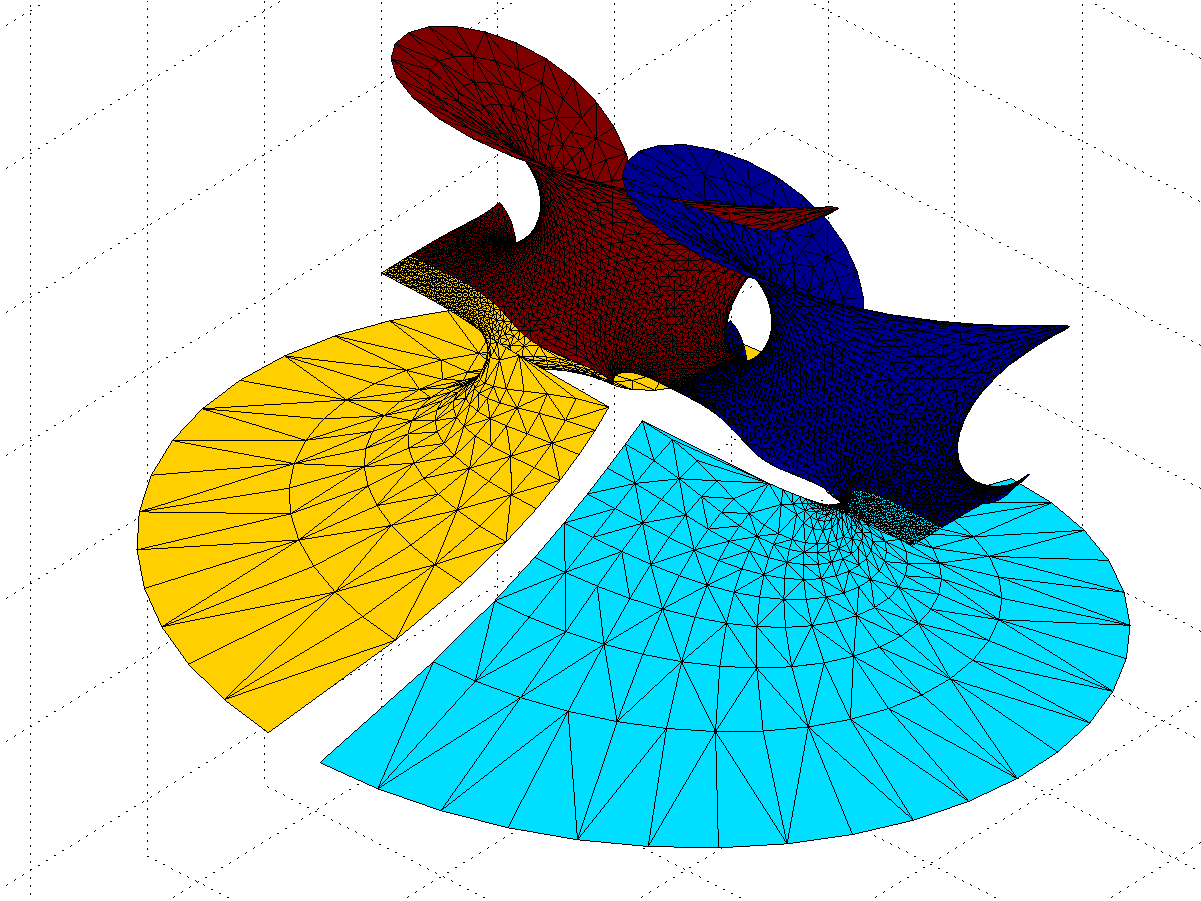
 . They also introduce residues along the y-direction, but different ones from the z=0 – their extensions of the surface will be out of phase with each other, making the fully extended surface fantastically self-intersecting and confusing.
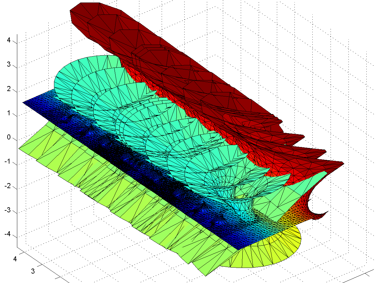
") is nicely behaved and looks very much like the Enneper surface near zero, with “wings” that oscillate ever more wildly as we move towards the negative reals. No doubt there are other beautiful things to look for in the vicinity.
is nicely behaved and looks very much like the Enneper surface near zero, with “wings” that oscillate ever more wildly as we move towards the negative reals. No doubt there are other beautiful things to look for in the vicinity.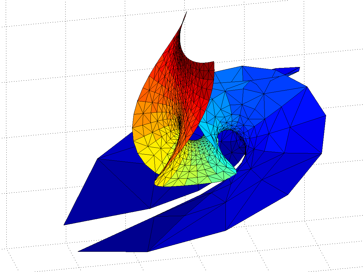

=\int_0^\infty t^{z-1}e^{-t} dt") , the continuous generalization of the factorial. While it grows rapidly for positive reals, it has fun poles for the negative integers and is generally complex.
, the continuous generalization of the factorial. While it grows rapidly for positive reals, it has fun poles for the negative integers and is generally complex. ") . The result is a nice fractal, with some domains approaching 1, and others running off to infinity.
. The result is a nice fractal, with some domains approaching 1, and others running off to infinity.
 . Zooming in a bit more reveals neat self-similar patterns with alternating “beans”:
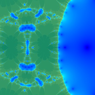

") where c is the control parameter. I start with
where c is the control parameter. I start with 


 operations per second, or somewhere in the zettaFLOPS range
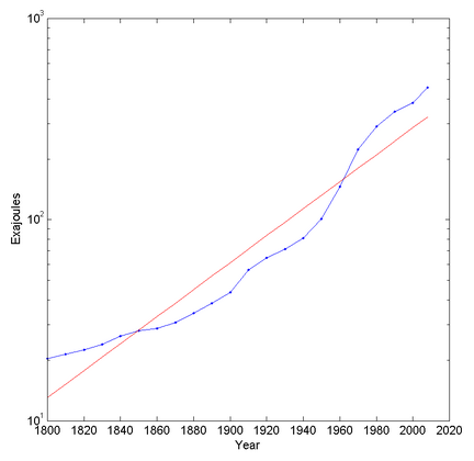
") joules of energy have to be dissipated. Given current efficiency trends we will reach this limit around 2048.
joules of energy have to be dissipated. Given current efficiency trends we will reach this limit around 2048. = \exp(kt) = P(t)/M(t)") , where
, where ") is the power of the system and
is the power of the system and ") is the mass of the system at time t. One can maintain exponential growth by reducing the mass as well as increasing the power.
is the mass of the system at time t. One can maintain exponential growth by reducing the mass as well as increasing the power. radiates it away into space, then the temperature will be
 ![T=[\rho \Phi R/3 \sigma]^{1/4}](https://s0.wp.com/latex.php?latex=T%3D%5B%5Crho+%5CPhi+R%2F3+%5Csigma%5D%5E%7B1%2F4%7D&bg=ffffff&fg=000000&s=0 "T=[\rho \Phi R/3 \sigma]^{1/4}") , or, if we have a maximal acceptable temperature,
, or, if we have a maximal acceptable temperature,  . So the system needs to become smaller as
  increases. If we use active heat transport instead (
 . Again, the radius will be inversely proportional to
 ![I = P/kT \ln(2) = \Phi M / kT\ln(2) = [4 \pi \rho /3 k \ln(2)] \Phi R^3 / T](https://s0.wp.com/latex.php?latex=I+%3D+P%2FkT+%5Cln%282%29+%3D+%5CPhi+M+%2F+kT%5Cln%282%29+%3D+%5B4+%5Cpi+%5Crho+%2F3+k+%5Cln%282%29%5D+%5CPhi+R%5E3+%2F+T&bg=ffffff&fg=000000&s=0 "I = P/kT \ln(2) = \Phi M / kT\ln(2) = [4 \pi \rho /3 k \ln(2)] \Phi R^3 / T") bits per second. Using the first cooling model gives us
bits per second. Using the first cooling model gives us  – a massive advantage for running extremely hot and dense computation. In the second cooling model
  : in both cases higher energy rate densities make it harder to compute when close to the thermodynamic limit. Hence there might be an upper limit to how much we may want to push
  : the higher the rate, the faster it will run out (and it is independent of size!). If the system is expanding at speed v it will gain and use up mass at a rate
 /c^2") ; if
; if  where
where  bits per kg per meter), and we only have access to a volume
  with mass density
  . It grows quickly, but still just polynomially.
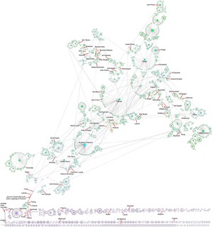