One of the first fractals I ever saw was the Apollonian gasket, the shape that emerges if you draw the circle internally tangent to three other tangent circles. It is somewhat similar to the Sierpinski triangle, but has a more organic flair. I can still remember opening my copy of Mandelbrot’s The Fractal Geometry of Nature and encountering this amazing shape. There is a lot of interesting things going on here.
Here is a simple algorithm for generating related circle packings, trading recursion for flexibility:
Start with a domain and calculate the distance to the border for all interior points.
Place a circle of radius at the point with maximal distance from the border.
Recalculate the distances, treating the new circle as a part of the border.
Repeat (2-3) until the radius becomes smaller than some tolerance.
This is easily implemented in Matlab if we discretize the domain and use an array of distances , which is then updated where is the distance to the circle. This trades exactness for some discretization error, but it can easily handle nearly arbitrary shapes.
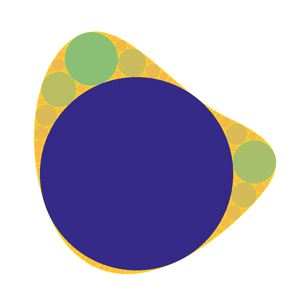
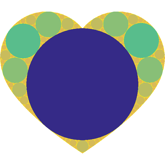
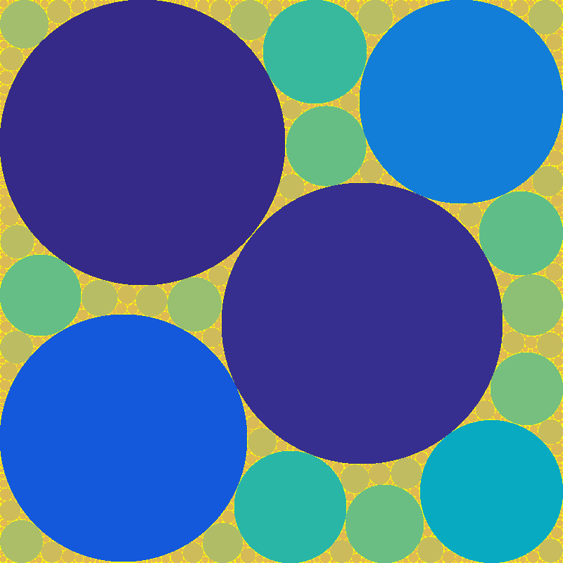
Apollonian circle packing in square.Apollonian circle packing in blob.Apollonian circle packing in heart.
It is interesting to note that the topology is Apollonian nearly everywhere: as soon as three circles form a curvilinear triangle the interior will be a standard gasket if .
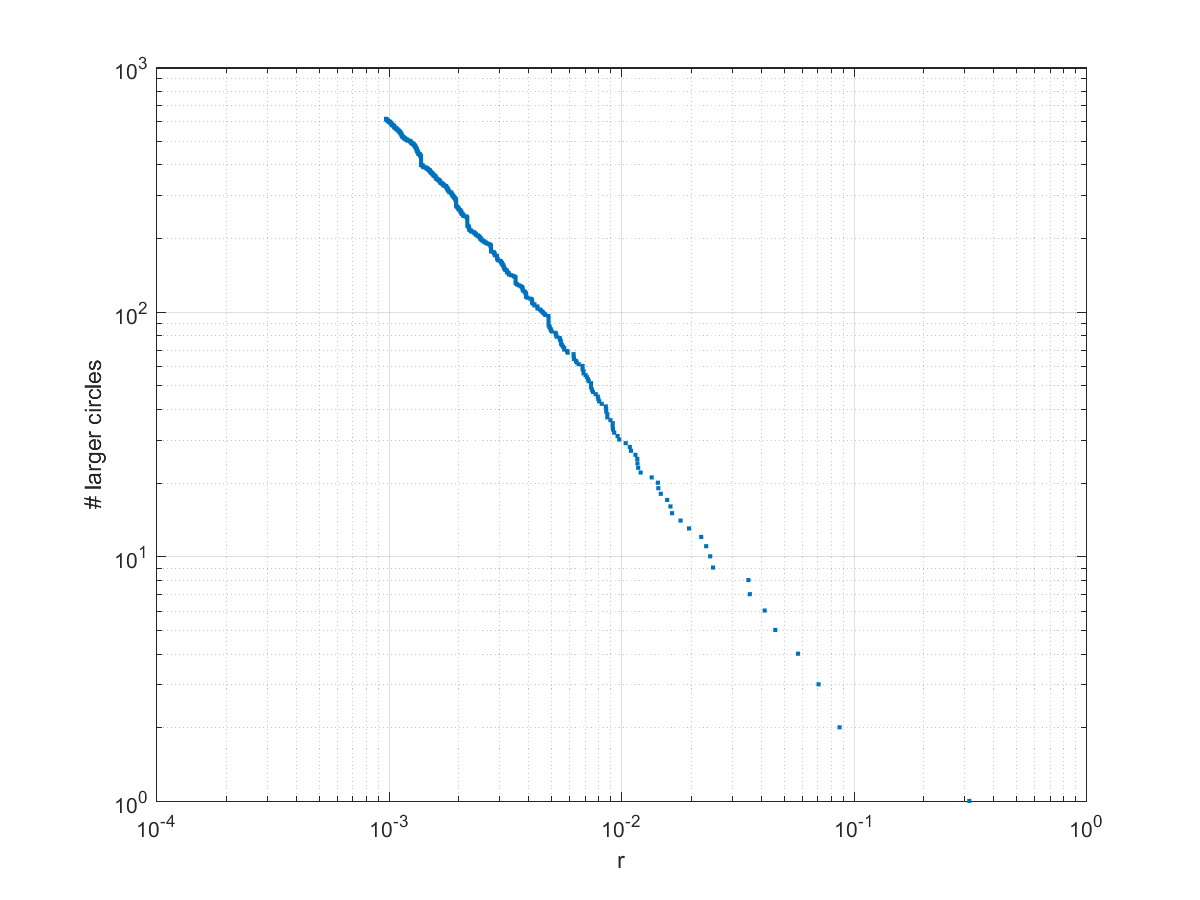
Number of circles larger than a certain radius in packing in blob shape.
In the above pictures the first circle tends to dominate. In fact, the size distribution of circles is a power law: the number of circles larger than r grows as as we approach zero, with . This is unsurprising: given a generic curved triangle, the inscribed circle will be a fraction of the radii of the bordering circles. If one looks at integral circle packings it is possible to see that the curvatures of subsequent circles grow quadratically along each “horn”, but different “horns” have different growths. Because of the curvature the self-similarity is nontrivial: there is actually, as far as I know, still no analytic expression of the fractal dimension of the gasket. Still, one can show that the packing exponent is the Hausdorff dimension of the gasket.
Anyway, to make the first circle less dominant we can either place a non-optimal circle somewhere, or use lower .
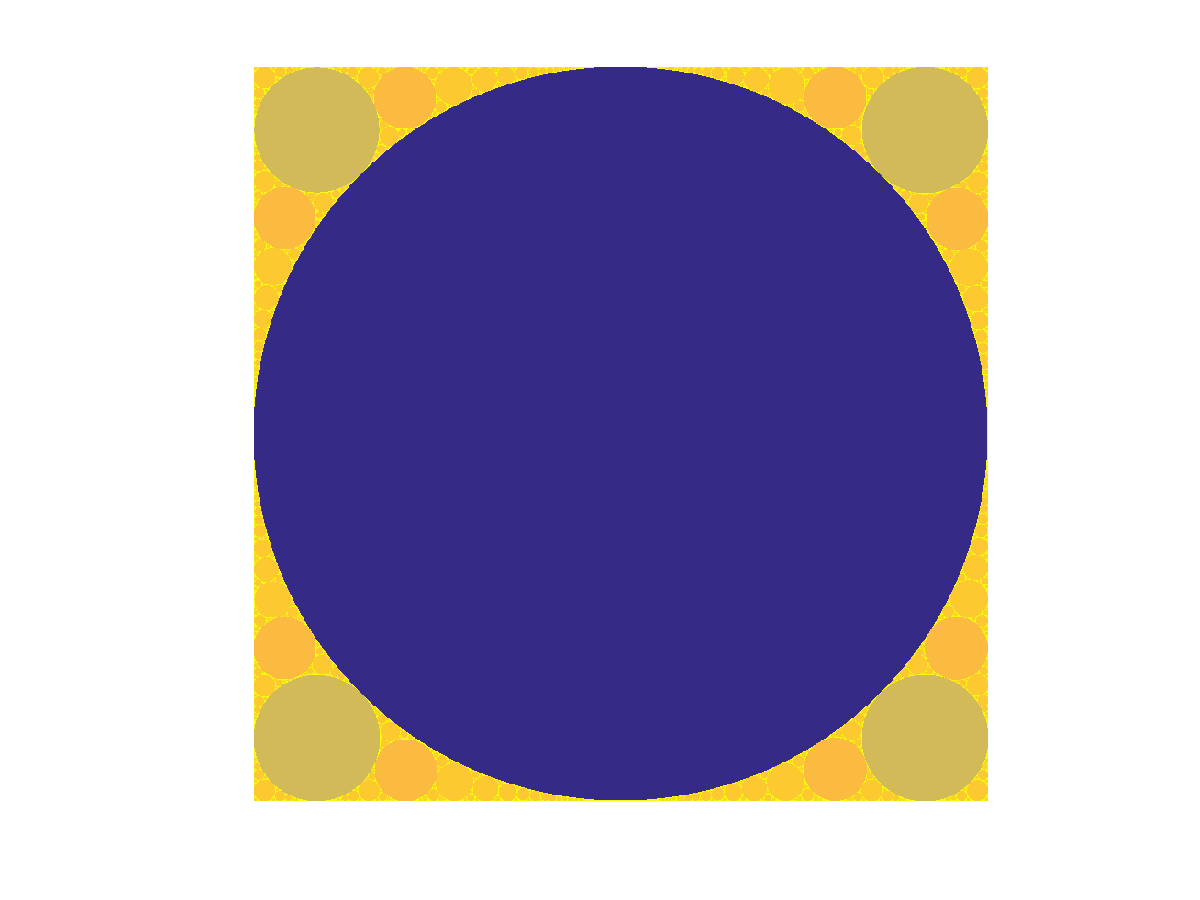
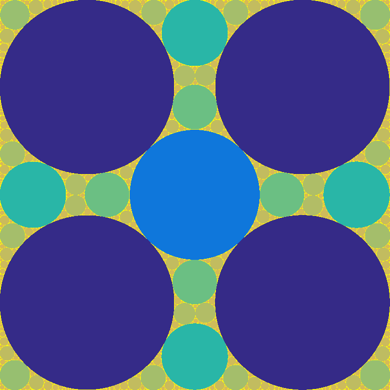
Apollonian packing in square with central circle of radius 1/6.
If we place a circle in the centre of a square with a radius smaller than the distance to the edge, it gets surrounded by larger circles.
Randomly started Apollonian packing.
If the circle is misaligned, it is no problem for the tiling: any discrepancy can be filled with sufficiently small circles. There is however room for arbitrariness: when a bow-tie-shaped region shows up there are often two possible ways of placing a maximal circle in it, and whichever gets selected breaks the symmetry, typically producing more arbitrary bow-ties. For “neat” arrangements with the right relationships between circle curvatures and positions this does not happen (they have circle chains corresponding to various integer curvature relationships), but the generic case is a mess. If we move the seed circle around, the rest of the arrangement both show random jitter and occasional large-scale reorganizations.
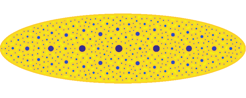
When we let we get sponge-like fractals: these are relatives to the Menger sponge and the Cantor set. The domain gets an infinity of circles punched out of itself, with a total area approaching the area of the domain, so the total measure goes to zero.
Apollonian packing with alpha=0.5.
That these images have an organic look is not surprising. Vascular systems likely grow by finding the locations furthest away from existing vascularization, then filling in the gaps recursively (OK, things are a bit more complex).
Apollonian packing with alpha=1/4.Apollonian packing with alpha=0.1.
Recently I encountered a specialist Wiki. I pressed “random page” a few times, and got a repeat page after 5 tries. How many pages should I expect this small wiki to have?
We can compare this to the German tank problem. Note that it is different; in the tank problem we have a maximum sample (maybe like the web pages on the site were numbered), while here we have number of samples before repetition.
We can of course use Bayes theorem for this. If I get a repeat after random samples, the posterior distribution of , the number of pages, is .
If I randomly sample from pages, the probability of getting a repeat on my second try is , on my third try , and so on: . Of course, there has to be more pages than , otherwise a repeat must have happened before step , so this is valid for . Otherwise, for .
The prior needs to be decided. One approach is to assume that websites have a power-law distributed number of pages. The majority are tiny, and then there are huge ones like Wikipedia; the exponent is close to 1. This gives us . Note the appearance of the Riemann zeta function as a normalisation factor.
We can calculate by summing over the different possible : .
Putting it all together we get for . The posterior distribution of number of pages is another power-law. Note that the dependency on is rather subtle: it is in the support of the distribution, and the upper limit of the partial sum.
What about the expected number of pages in the wiki? . The expectation is the ratio of the zeta functions of and , minus the first terms of their series.
Distribution of P(N|5) for [latex]\alpha=1.1[/latex].
So, what does this tell us about the wiki I started with? Assuming (close to the behavior of big websites), it predicts . If one assumes a higher the number of pages would be 7 (which was close to the size of the wiki when I looked at it last night – it has grown enough today for k to equal 13 when I tried it today).
Expected number of pages given k random views before a repeat.
So, can we derive a useful rule of thumb for the expected number of pages? Dividing by shows that approaches proportionality, especially for larger :
E(N|k)/k as a function of k.
So a good rule of thumb is that if you get pages before a repeat, expect between and pages on the site. However, remember that we are dealing with power-laws, so the variance can be surprisingly high.
Yesterday I gave a talk at the joint Bloomberg-London Futurist meeting “The state of the future” about the future of decisionmaking. Parts were updates on my policymaking 2.0 talk (turned into this chapter), but I added a bit more about individual decisionmaking, rationality and forecasting.
The big idea of the talk: ensemble methods really work in a lot of cases. Not always, not perfectly, but they should be among the first tools to consider when trying to make a robust forecast or decision. They are Bayes’ broadsword:
OK, so in forecasting it looks like using multiple methods, theories and data sources (including experts) is a way to get better results.
Statistical machine learning
A standard problem in machine learning is to classify something into the right category from data, given a set of training examples. For example, given medical data such as age, sex, and blood test results, diagnose what a particular disease a patient might suffer from. The key problem is that it is non-trivial to construct a classifier that works well on data different from the training data. It can work badly on new data, even if it works perfectly on the training examples. Two classifiers that perform equally well during training may perform very differently in real life, or even for different data.
The obvious solution is to combine several classifiers and average (or vote about) their decisions: ensemble based systems. This reduces the risk of making a poor choice, and can in fact improve overall performance if they can specialize for different parts of the data. This also has other advantages: very large datasets can be split into manageable chunks that are used to train different components of the ensemble, tiny datasets can be “stretched” by random resampling to make an ensemble trained on subsets, outliers can be managed by “specialists”, in data fusion different types of data can be combined, and so on. Multiple weak classifiers can be combined into a strong classifier this way.
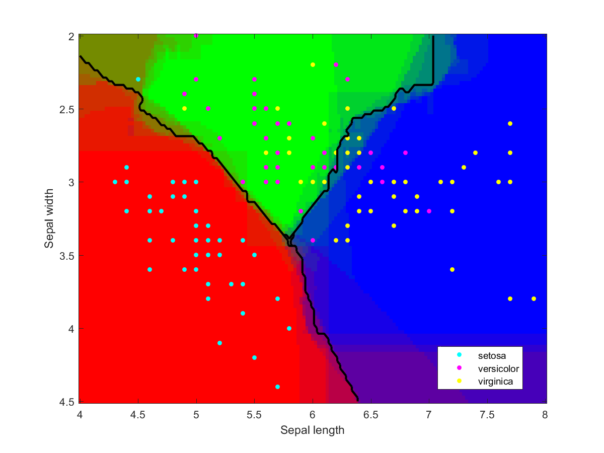
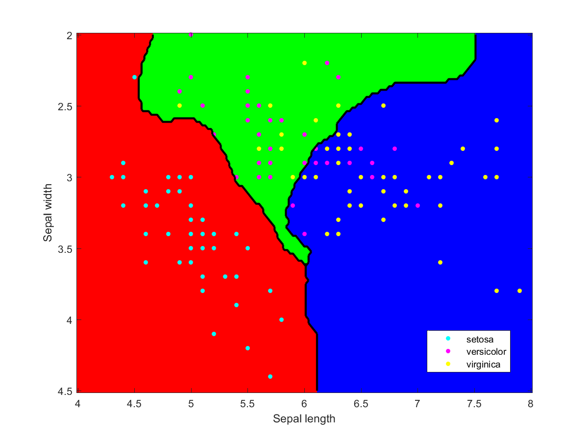
Iris data classified using an ensemble of classification methods (LDA, NBC, various kernels, decision tree). Note how the combination of classifiers also roughly indicates the overall reliability of classifications in a region.
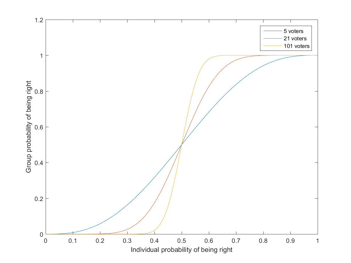
Condorcet’s jury theorem is perhaps the classic result in group problem solving: if a group of people hold a majority vote, and each has a probability p>1/2 of voting for the correct choice, then the probability the group will vote correctly is higher than p and will tend to approach 1 as the size of the group increases. This presupposes that votes are independent, although stronger forms of the theorem have been proven. (In reality people may have different preferences so there is no clear “right answer”)
Probability that groups of different sizes will reach the correct decision as a function of the individual probability of voting right.
By now the pattern is likely pretty obvious. Weak decision-makers (the voters) are combined through a simple procedure (the vote) into better decision-makers.
Group problem solving is known to be pretty good at smoothing out individual biases and errors. In The Wisdom of Crowds Surowiecki suggests that the ideal crowd for answering a question in a distributed fashion has diversity of opinion, independence (each member has an opinion not determined by the other’s), decentralization (members can draw conclusions based on local knowledge), and the existence of a good aggregation process turning private judgements into a collective decision or answer.
Perhaps the grandest example of group problem solving is the scientific process, where peer review, replication, cumulative arguments, and other tools make error-prone and biased scientists produce a body of findings that over time robustly (if sometimes slowly) tends towards truth. This is anything but independent: sometimes a clever structure can improve performance. However, it can also induce all sorts of nontrivial pathologies – just consider the detrimental effects status games have on accuracy or focus on the important topics in science.
Small group problem solving on the other hand is known to be great for verifiable solutions (everybody can see that a proposal solves the problem), but unfortunately suffers when dealing with “wicked problems” lacking good problem or solution formulation. Groups also have scaling issues: a team of N people need to transmit information between all N(N-1)/2 pairs, which quickly becomes cumbersome.
One way of fixing these problems is using software and formal methods.
The Good Judgement Project (partially run by Tetlock and with Armstrong on the board of advisers) participated in the IARPA ACE program to try to improve intelligence forecasts. They used volunteers and checked their forecast accuracy (not just if they got things right, but if claims that something was 75% likely actually came true 75% of the time). This led to a plethora of fascinating results. First, accuracy scores based on the first 25 questions in the tournament predicted subsequent accuracy well: some people were consistently better than others, and it tended to remain constant. Training (such a debiasing techniques) and forming teams also improved performance. Most impressively, using the top 2% “superforecasters” in teams really outperformed the other variants. The superforecasters were a diverse group, smart but by no means geniuses, updating their beliefs frequently but in small steps.
The key to this success was that a computer- and statistics-aided process found the good forecasters and harnessed them properly (plus, the forecasts were on a shorter time horizon than the policy ones Tetlock analysed in his previous book: this both enables better forecasting, plus the all-important feedback on whether they worked).
Another good example is the Galaxy Zoo, an early crowd-sourcing project in galaxy classification (which in turn led to the Zooniverse citizen science project). It is not just that participants can act as weak classifiers and combined through a majority vote to become reliable classifiers of galaxy type. Since the type of some galaxies is agreed on by domain experts they can used to test the reliability of participants, producing better weightings. But it is possible to go further, and classify the biases of participants to create combinations that maximize the benefit, for example by using overly “trigger happy” participants to find possible rare things of interest, and then check them using both conservative and neutral participants to become certain. Even better, this can be done dynamically as people slowly gain skill or change preferences.
The right kind of software and on-line “institutions” can shape people’s behavior so that they form more effective joint cognition than they ever could individually.
Conclusions
The big idea here is that it does not matter that individual experts, forecasting methods, classifiers or team members are fallible or biased, if their contributions can be combined in such a way that the overall output is robust and less biased. Ensemble methods are examples of this.
While just voting or weighing everybody equally is a decent start, performance can be significantly improved by linking it to how well the participants perform. Humans can easily be motivated by scoring (but look out for disalignment of incentives: the score must accurately reflect real performance and must not be gameable).
Having a flexible structure that can change is a good approach to handling a changing world. If people have disincentives to change their mind or change teams, they will not update beliefs accurately.
I got a good question after the talk: if we are supposed to keep our models simple, how can we use these complicated ensembles? The answer is of course that there is a difference between using a complex and a complicated approach. The methods that tend to be fragile are the ones with too many free parameters, too much theoretical burden: they are the complex “hedgehogs”. But stringing together a lot of methods and weighting them appropriately merely produces a complicated model, a “fox”. Component hedgehogs are fine as long as they are weighed according to how well they actually perform.
(In fact, adding together many complex things can make the whole simpler. My favourite example is the fact that the Kolmogorov complexity of integers grows boundlessly on average, yet the complexity of the set of all integers is small – and actually smaller than some integers we can easily name. The whole can be simpler than its parts.)
In the end, we are trading Occam’s razor for a more robust tool: Bayes’ Broadsword. It might require far more strength (computing power/human interaction) to wield, but it has longer reach. And it hits hard.
Appendix: individual classifiers
I used Matlab to make the illustration of the ensemble classification. Here are some of the component classifiers. They are all based on the examples in the Matlab documentation. My ensemble classifier is merely a maximum vote between the component classifiers that assign a class to each point.
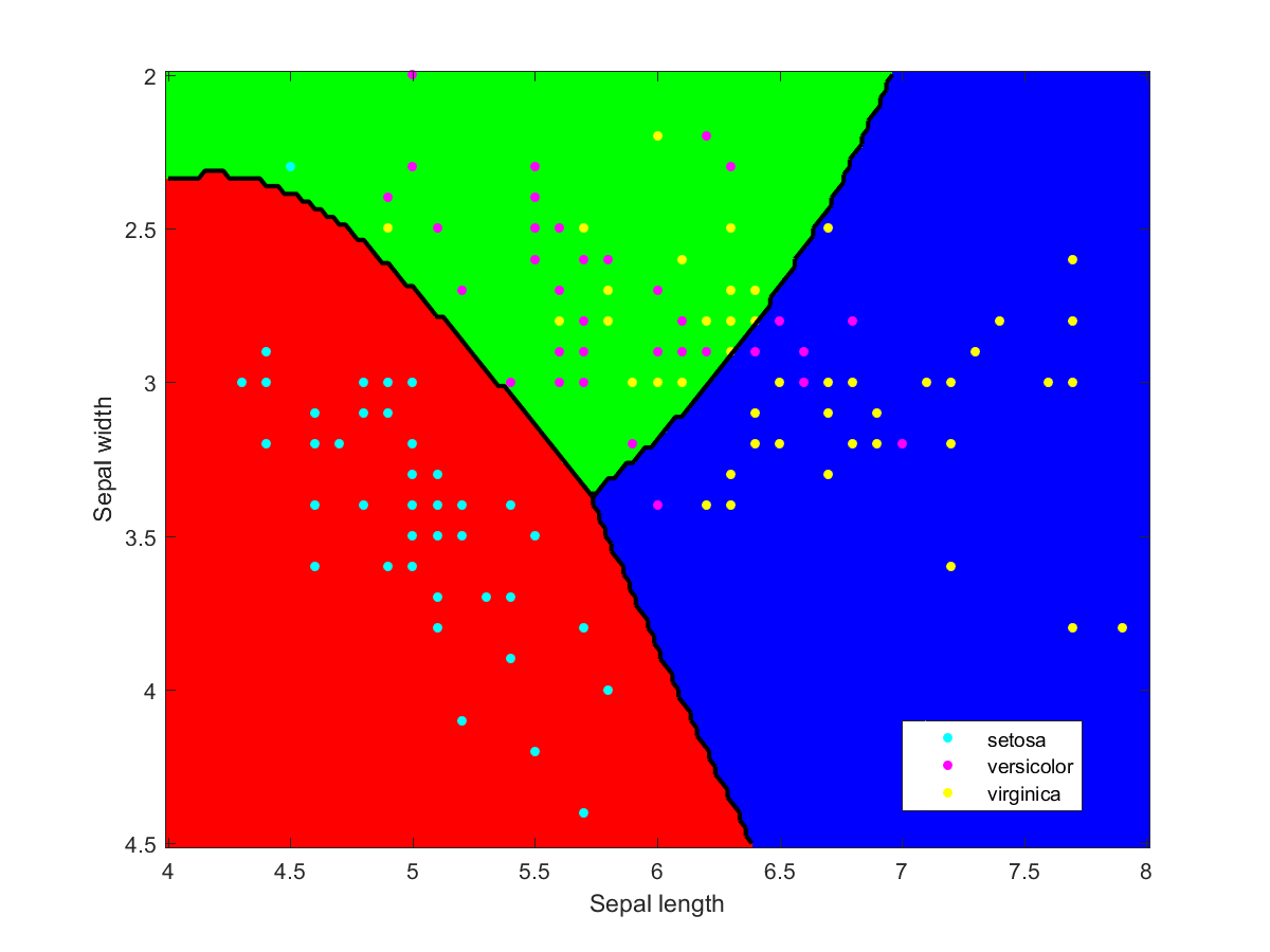
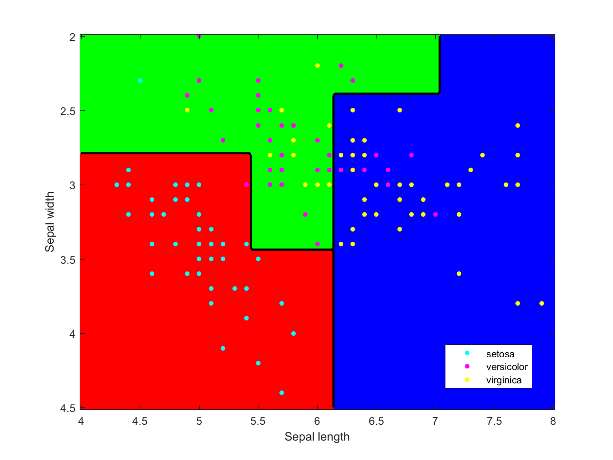
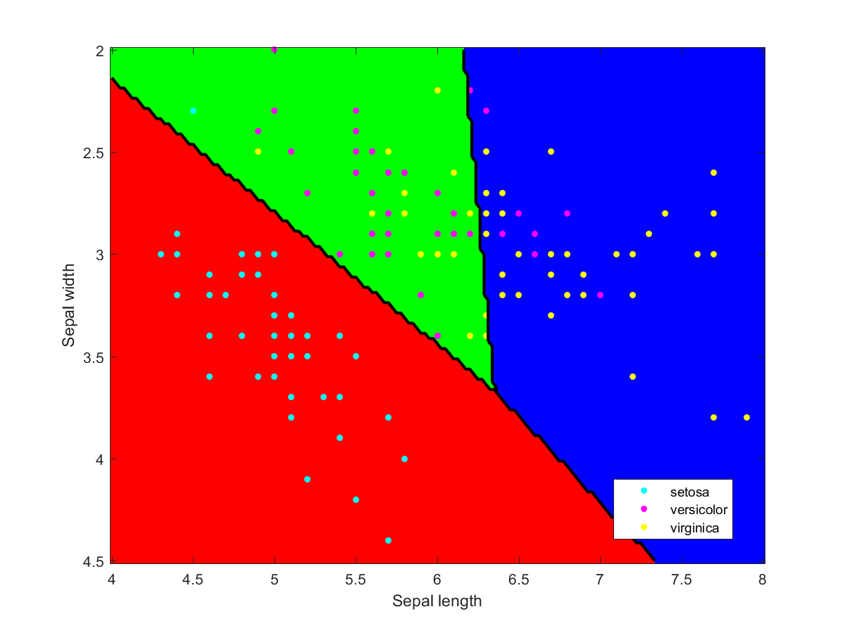
Iris data classified using a naive Bayesian classifier assuming Gaussian distributions.Iris data classified using a decision tree.Iris data classified using Gaussian kernels.Iris data classified using linear discriminant analysis.
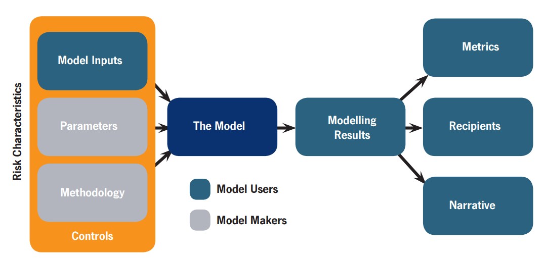
The basic story is that in insurance (and many other domains) people use statistical models to estimate risk, and then use these estimates plus human insight to come up with prices and decisions. It is well known (at least in insurance) that there is a measure of model risk due to the models not being perfect images of reality; ideally the users will take this into account. However, in reality (1) people tend to be swayed by models, (2) they suffer from various individual and collective cognitive biases making their model usage imperfect and correlates their errors, (3) the markets for models, industrial competition and regulation leads to fewer models being used than there could be. Together this creates a systemic risk: everybody makes correlated mistakes and decisions, which means that when a bad surprise happens – a big exogenous shock like a natural disaster or a burst of hyperinflation, or some endogenous trouble like a reinsurance spiral or financial bubble – the joint risk of a large chunk of the industry failing is much higher than it would have been if everybody had had independent, uncorrelated models. Cue bailouts or skyscrapers for sale.
Note that this is a generic problem. Insurance is just unusually self-aware about its limitations (a side effect of convincing everybody else that Bad Things Happen, not to mention seeing the rest of the financial industry running into major trouble). When we use models the model itself (the statistics and software) is just one part: the data fed into the model, the processes of building and tuning the model, how people use it in their everyday work, how the output leads to decisions, and how the eventual outcomes become feedback to the people involved – all of these factors are important parts in making model use useful. If there is no or too slow feedback people will not learn what behaviours are correct or not. If there are weak incentives to check errors of one type, but strong incentives for other errors, expect the system to become biased towards one side. It applies to climate models and military war-games too.
The key thing is to recognize that model usefulness is not something that is directly apparent: it requires a fair bit of expertise to evaluate, and that expertise is also not trivial to recognize or gain. We often compare models to other models rather than reality, and a successful career in predicting risk may actually be nothing more than good luck in avoiding rare but disastrous events.
What can we do about it? We suggest a scorecard as a first step: comparing oneself to some ideal modelling process is a good way of noticing where one could find room for improvement. The score does not matter as much as digging into one’s processes and seeing whether they have cruft that needs to be fixed – whether it is following standards mindlessly, employees not speaking up, basing decisions on single models rather than more broad views of risk, or having regulators push one into the same direction as everybody else. Fixing it may of course be tricky: just telling people to be less biased or to do extra error checking will not work, it has to be integrated into the organisation. But recognizing that there may be a problem and getting people on board is a great start.
If we wanted to represent humanity most honestly to aliens, we would just give them a constantly updated full documentation of our cultures and knowledge. But that is not possible.
So in METI we may consider sending “a copy of the internet” as a massive snapshot of what we currently are, or as the Voyager recording did, send a sample of what we are. In both cases it is a snapshot at a particular time: had we sent the message at some other time, the contents would have been different. The selection used is also a powerful shaper, with what is chosen as representative telling a particular story.
That we send a snapshot is not just a necessity, it may be a virtue. The full representation of what humanity is, is not so much a message as a gift with potentially tricky moral implications: imagine if we were given the record of an alien species, clearly sent with the intention that we ought to handle it according to some – to us unknowable – preferences. If we want to do some simple communication, essentially sending a postcard-like “here we are! This is what we think we are!” is the best we can do. A thick and complex message would obscure the actual meaning:
The spacecraft will be encountered and the record played only if there are advanced space-faring civilizations in interstellar space. But the launching of this ‘bottle’ into the cosmic ‘ocean’ says something very hopeful about life on this planet.
– Carl Sagan
It is a time capsule we send because we hope to survive and matter. If it becomes an epitaph of our species it is a decent epitaph. Anybody receiving it is a bonus.
Temporal preferences
How should we relate to this already made and launched message?
Clearly we want the message to persist, maybe be detected, and ideally understood. We do not want the message to be distorted by random chance (if it can be avoided) or by independent actors.
This is why I am not too keen on sending an addendum. One can change the meaning of a message with a small addition: “Haha, just kidding!” or “We were such tools in the 1970s!”
Note that we have a present desire for a message (possibly the original) to reach the stars, but the launchers in 1977 clearly wanted their message to reach the stars: their preferences were clearly linked to what they selected. I think we have a moral duty to respect past preferences for information. I have expressed it elsewhere as a temporal golden rule: “treat the past as you want the future to treat you”. We would not want our message or amendments changed, so we better be careful about past messages.
Additive additions
However, adding a careful footnote is not necessarily wrong. But it needs to be in the spirit of the past message, adding to it.
So what kind of update would be useful?
We might want to add something that we have learned since the launch that aliens ought to know. For example, an important discovery. But this needs to be something that advanced aliens are unlikely to already know, which is tricky: they likely know about dark matter, that geopolitical orders can suddenly shift, or a proof of the Poincaré conjecture.
They have to be contingent, unique to humanity, and ideally universally significant. Few things are. Maybe that leaves us with adding the notes for some new catchy melody (“Gangnam style” or “Macarena”?) or a really neat mathematical insight (PCP theorem? Oops, it looks like Andrew Wiles’ Fermat proof is too large for the probe).
In the end, maybe just a “Still here, 38 years later” may be the best addition. Contingent, human, gives some data on the survival of intelligence in the universe.
at the point with maximal distance
from the border.
")
 \leftarrow \min(d(x,y), D(x,y))")
")

\propto r^-\delta")


 random samples, the posterior distribution of
  , the number of pages, is
  = P(k|N)P(N)/P(k)") .
. , on my third try
  , and so on:
 =(k-1)/N") . Of course, there has to be more pages than
. Of course, there has to be more pages than  , otherwise a repeat must have happened before step
  . Otherwise,
 =0") for
for  .
.") needs to be decided. One approach is to assume that websites have
needs to be decided. One approach is to assume that websites have  = N^{-\alpha}/\zeta(\alpha)") . Note the appearance of the Riemann zeta function as a normalisation factor.
. Note the appearance of the Riemann zeta function as a normalisation factor.") by summing over the different possible
by summing over the different possible =\sum_{N=1}^\infty P(k|N)P(N) = \frac{k-1}{\zeta(\alpha)}\sum_{N=k-1}^\infty N^{-(\alpha+1)}")
}(\zeta(\alpha+1)-\sum_{i=1}^{k-2}i^{-(\alpha+1)})") .
.=N^{-(\alpha+1)}/(\zeta(\alpha+1) -\sum_{i=1}^{k-2}i^{-(\alpha+1)})") for
for  . The posterior distribution of number of pages is another power-law. Note that the dependency on
 =\sum_{N=1}^\infty N P(N|k) = \sum_{N=k-1}^\infty N^{-\alpha}/(\zeta(\alpha+1) -\sum_{i=1}^{k-2}i^{-(\alpha+1)})")
-\sum_{i=1}^{k-2} i^{-\alpha}}{\zeta(\alpha+1)-\sum_{i=1}^{k-2}i^{-(\alpha+1)}}") . The expectation is the ratio of the zeta functions of
. The expectation is the ratio of the zeta functions of  , minus the first
  terms of their series.
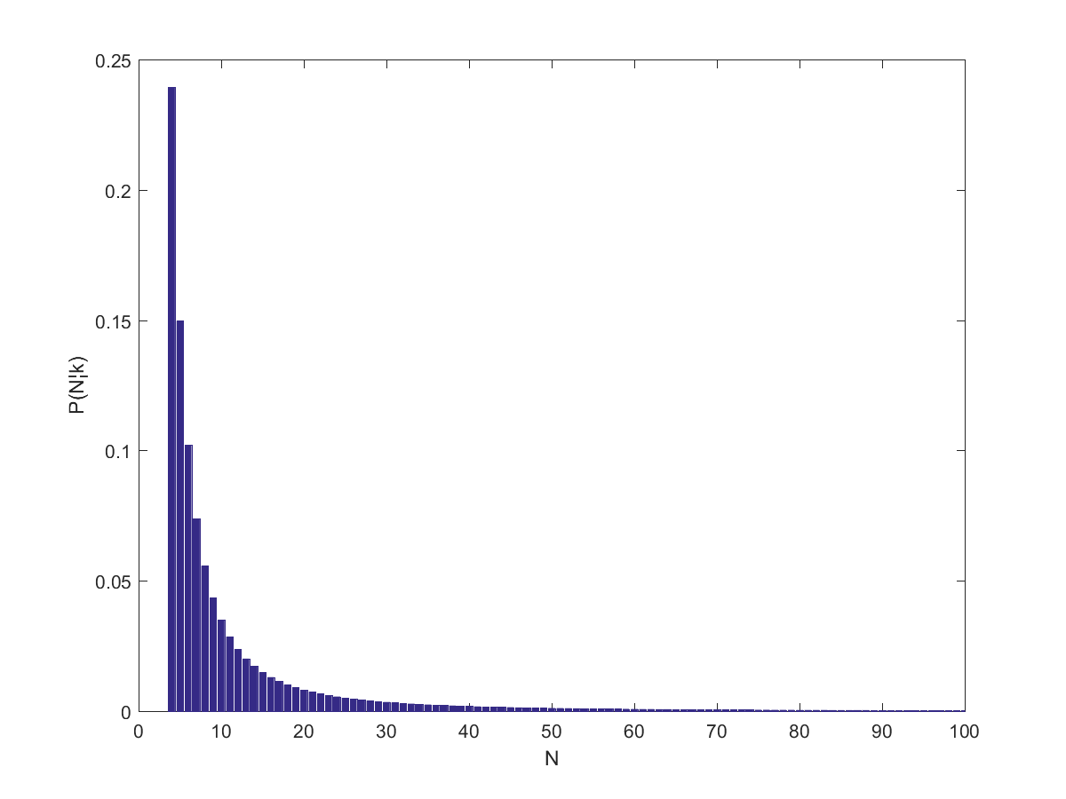
 (close to the behavior of big websites), it predicts
 \approx 21.28") . If one assumes a higher
. If one assumes a higher  the number of pages would be 7 (which was close to the size of the wiki when I looked at it last night – it has grown enough today for k to equal 13 when I tried it today).
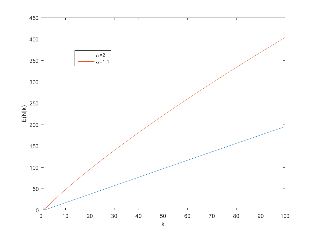
") approaches proportionality, especially for larger
approaches proportionality, especially for larger 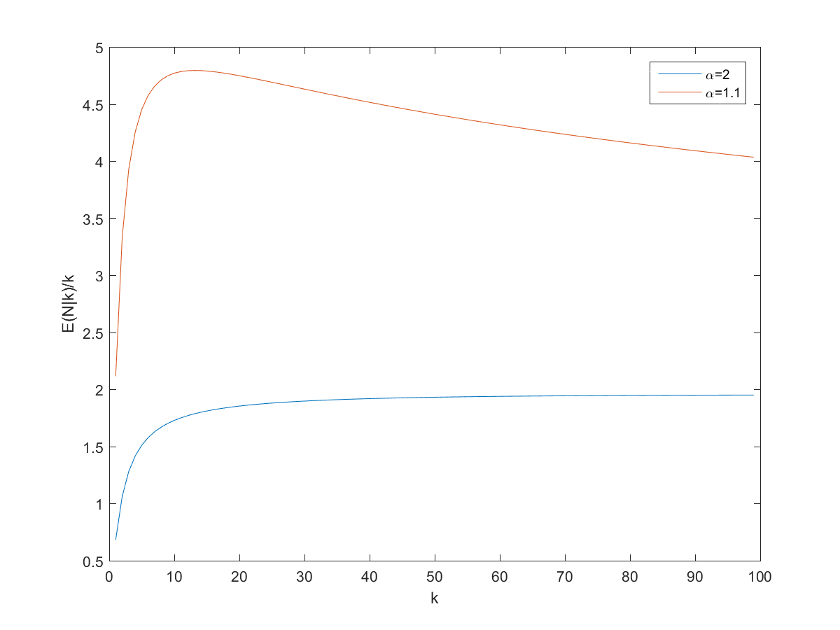
 and
and  pages on the site. However, remember that we are dealing with power-laws, so the variance can be surprisingly high.