A great question from twitter:
Food for thought: There exists some smallest whole number which no human will ever think about.
I wonder how big it is.
— Grant Sanderson (@3blue1brown) January 6, 2020
This is a bit like the “what is the smallest uninteresting number?” paradox, but not paradoxical: we do not have to name it (and hence make it thought about/interesting) to reason about it.
I will first give a somewhat rough probabilistic bound, and then a much easier argument for the scale of this number. TL;DR: the number is likely smaller than 
Probabilistic bound
If we think about 
")
")

If we denote the cumulative distribution function ![P(x)=\Pr[X<x]](https://s0.wp.com/latex.php?latex=P%28x%29%3D%5CPr%5BX%3Cx%5D&bg=ffffff&fg=000000&s=0 "P(x)=\Pr[X<x]")
![F_{(k)}(x) = [P(x)]^{k}](https://s0.wp.com/latex.php?latex=F_%7B%28k%29%7D%28x%29+%3D+%5BP%28x%29%5D%5E%7Bk%7D&bg=ffffff&fg=000000&s=0 "F_{(k)}(x) = [P(x)]^{k}")
}(x^*)=1/2")
What shape does \sim 1/\sqrt{x}")
So if we have 
=\frac{1}{2(k-1)}\frac{1}{\sqrt{x}}")
=(\sqrt{x}-1)/(k-1)")
![F_{(k)}(x)=[(\sqrt{x}-1)/(k-1)]^k](https://s0.wp.com/latex.php?latex=F_%7B%28k%29%7D%28x%29%3D%5B%28%5Csqrt%7Bx%7D-1%29%2F%28k-1%29%5D%5Ek&bg=ffffff&fg=000000&s=0 "F_{(k)}(x)=[(\sqrt{x}-1)/(k-1)]^k")
2^{-1/k}+1)^2 \approx k^2 - 2k \ln(2)")

So, how large is $k$ today? Dorogovtsev et al. had on the order of 

Consider a number…
Another approach is to assume each human considers a number about once a minute throughout their lifetime (clearly an overestimate given childhood, sleep, innumeracy etc. but we are mostly interested in orders of magnitude anyway and making an upper bound) which we happily assume to be about a century, giving a personal 


But that assumes “random” numbers, and is a very loose upper bound, merely describing a “typical” small unconsidered number. Were we to systematically think through the numbers from 1 and onward we would have the much lower 
One can refine this a bit: if we have time 


Seth Lloyd estimated that the observable universe cannot have performed more than 


This can be used to consider the future too. Computation of our kind can continue until proton decay in 
But the conclusion is clear: if you write a 173 digit number with no particular pattern of digits (a bit more than two standard lines of typing), it is very likely that this number would never have shown up across the history of the entire universe except for your action. And there is a smaller number that nobody – no human, no alien, no posthuman galaxy brain in the far future – will ever consider.
 , the number of pages, is
  = P(k|N)P(N)/P(k)") .
. , on my third try
  , and so on:
 =(k-1)/N") . Of course, there has to be more pages than
. Of course, there has to be more pages than  , otherwise a repeat must have happened before step
  . Otherwise,
 =0") for
for  .
.") needs to be decided. One approach is to assume that websites have
needs to be decided. One approach is to assume that websites have  = N^{-\alpha}/\zeta(\alpha)") . Note the appearance of the Riemann zeta function as a normalisation factor.
. Note the appearance of the Riemann zeta function as a normalisation factor.") by summing over the different possible
by summing over the different possible =\sum_{N=1}^\infty P(k|N)P(N) = \frac{k-1}{\zeta(\alpha)}\sum_{N=k-1}^\infty N^{-(\alpha+1)}")
}(\zeta(\alpha+1)-\sum_{i=1}^{k-2}i^{-(\alpha+1)})") .
.=N^{-(\alpha+1)}/(\zeta(\alpha+1) -\sum_{i=1}^{k-2}i^{-(\alpha+1)})") for
for  . The posterior distribution of number of pages is another power-law. Note that the dependency on
 =\sum_{N=1}^\infty N P(N|k) = \sum_{N=k-1}^\infty N^{-\alpha}/(\zeta(\alpha+1) -\sum_{i=1}^{k-2}i^{-(\alpha+1)})")
-\sum_{i=1}^{k-2} i^{-\alpha}}{\zeta(\alpha+1)-\sum_{i=1}^{k-2}i^{-(\alpha+1)}}") . The expectation is the ratio of the zeta functions of
. The expectation is the ratio of the zeta functions of  and
and  , minus the first
  terms of their series.
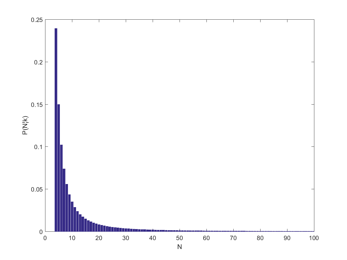
 (close to the behavior of big websites), it predicts
 \approx 21.28") . If one assumes a higher
. If one assumes a higher  the number of pages would be 7 (which was close to the size of the wiki when I looked at it last night – it has grown enough today for k to equal 13 when I tried it today).
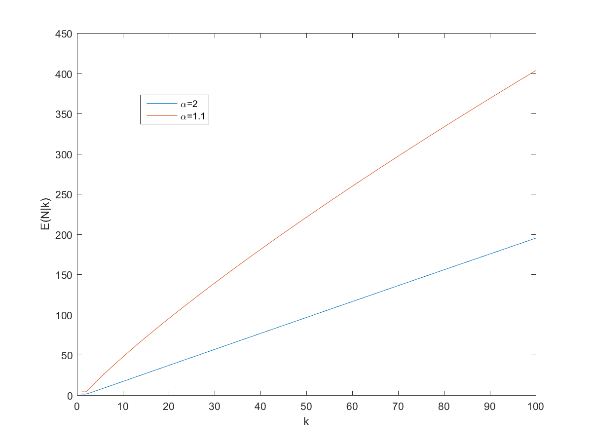
") approaches proportionality, especially for larger
approaches proportionality, especially for larger 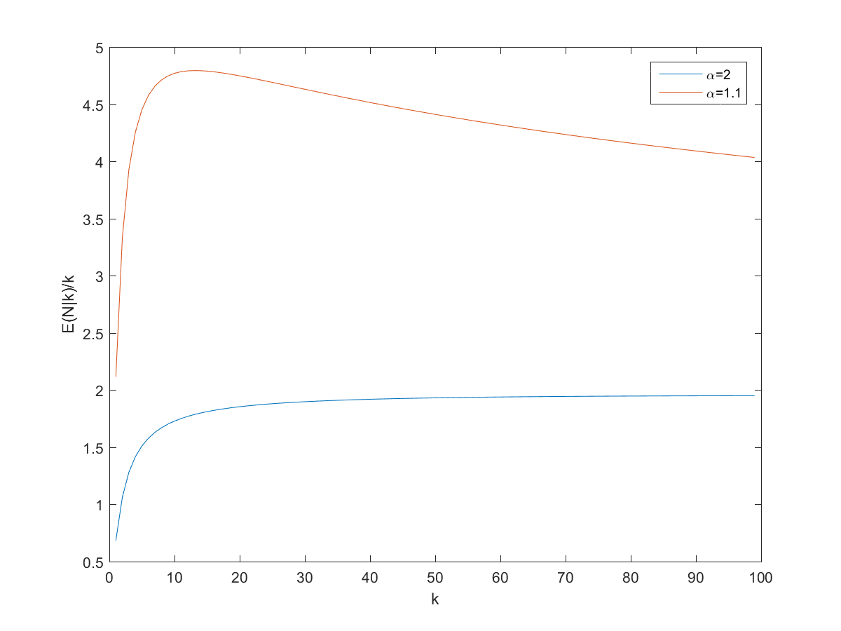
 and
and  pages on the site. However, remember that we are dealing with power-laws, so the variance can be surprisingly high.
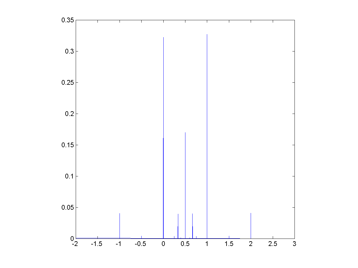
") and generate ratios
and generate ratios ") , then those ratios will have a distribution that is a convolution over the rational numbers:
, then those ratios will have a distribution that is a convolution over the rational numbers:  = g(a/(a+b)) = \sum_{m=0}^\infty \sum_{n=0}^\infty f(m) g(n) \delta \left(\frac{a}{a+b} - \frac{m}{m+n} \right ) = \sum_{t=0}^\infty f(ta)f(tb)")
 they get
 ) = (1/L^2) \lfloor L/\max(a,b) \rfloor") .
.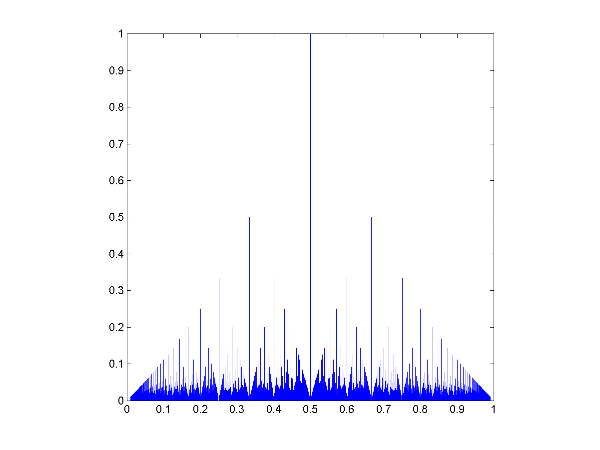
 where
where  :
:![The rational distribution of two convolved Exp[0.1] distributions.](http://aleph.se/andart2/wp-content/uploads/2014/09/trifonovexp01.png)
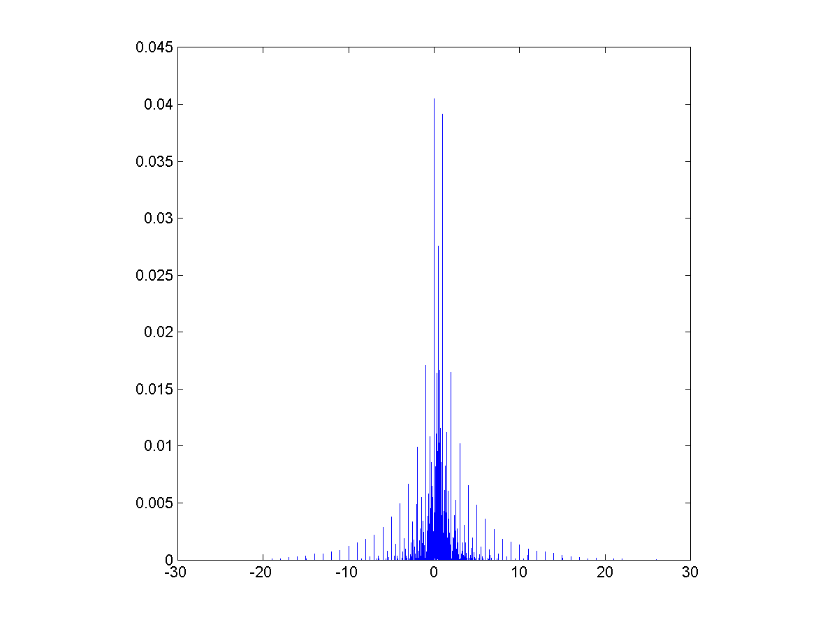
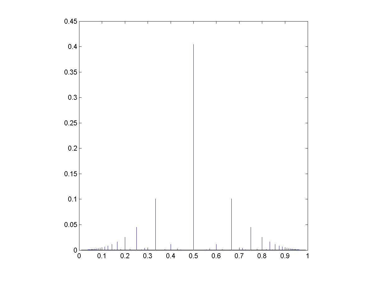
![Rational distribution of ratio between a Poisson[10] and a Poisson[5] variable.](http://aleph.se/andart2/wp-content/uploads/2014/09/trifonovpoiss105.png)