Quantifying busyness

Tempus fugit

If I have one piece of advice to give to people, it is that they typically have way more time now than they will ever have in the future. Do not procrastinate, take chances when you see them – you might never have the time to do it later.

One reason is the gradual speeding up of subjective time as we age: one day is less time for a 40 year old than for a 20 year old, and way less than the eon it is to a 5 year old. Another is that there is a finite risk that opportunities will go away (including our own finite lifespans). The main reason is of course the planning fallacy: since we underestimate how long our tasks will take, our lives tend to crowd up. Accepting to give a paper in several months time is easy, since there seems to be a lot of time to do it in between… which mysteriously disappears until you sit there doing an all-nighter. There is also the likely effect that as you grow in skill, reputation and career there will be more demands on your time. All in all, expect your time to grow in preciousness!

Mining my calendar

I recently noted that my calendar had filled up several weeks in advance, something I think did not happen to this extent a few years back. A sign of a career taking off, worsening time management, or just bad memory? I decided to do some self-quantification using my Google calendar. I exported the calendar as an .ics file and made a simple parser in Matlab.

Histogram of time distance between scheduling time and actual event.

It is pretty clear from a scatter plot that most entries are for the near future – a few days or weeks ahead. Looking at a histogram shows that most are within a month (a few are in the past – I sometimes use my calendar to note when I have done something like an interview that I may want to remember later).

Log-log plot of the histogram of event scheduling intervals.

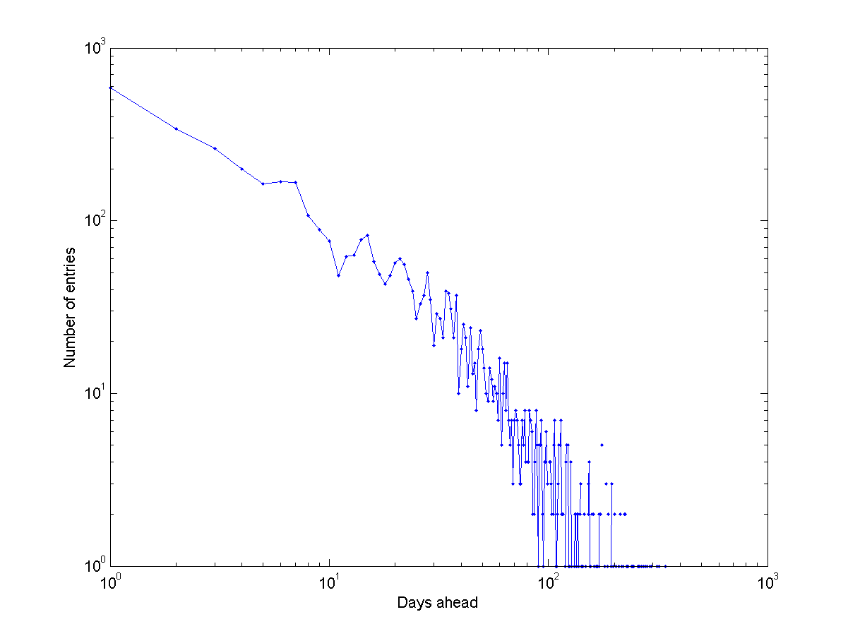
Plotting it as a log-log diagram suggests it is lighter-tailed than a power-law: there is a characteristic scale. And there are a few wobbles suggesting 1-week, 2-week and 3-week periodicities.

Mean and median distance to newly scheduled events (top), annual number of events scheduled (bottom). The eventual 2015 annual number has been estimated (dashed line).

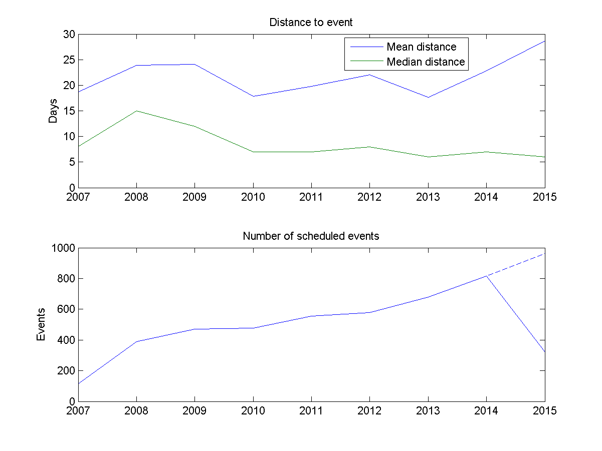
Am I getting busier? Plotting the mean and median distance to scheduled events, and the number of events per year, suggests yes. The median distance to the things I schedule seems to be creeping downwards, while the number of events per year has clearly doubled from about 400 in 2008 to 800 in 2014 (and extrapolating 2015 suggests about 1000 scheduled events).

Number of calendar events per 14 day period. Red line marks present.

Plotting the number of events I had per 14-day period also suggests that I have way more going on now than a few years ago. The peaks are getting higher and the mean period is more intense.

When am I free?

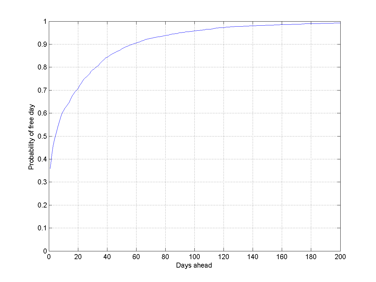
A good measure of busyness would be the time horizon: how far ahead should you ask me for a meeting if you want to have a high chance of getting it?

One approach would be to look for the probability $Q(t)$ that a day $t$ days ahead is entirely empty. If the probability that I will fill in something $i$ days ahead is $P(i)$ , then the chance for an empty day is $Q(t) = \prod_{i=t}^\infty (1-P(i))$ . We can estimate $P(i)$ by doing a curve-fit (a second degree curve works well), but we can of course just estimate from the histogram counts: $\hat{P}(i)=N(i)/N$ .

Probability that I will have an entirely free day a certain number of days ahead.

However, this method is slightly wrong. Some days are free, others have many different events. If I schedule twice as many events the chance of a free day should be lower. A better way of estimating $Q(t)$ is to think in terms of the rate of scheduling. We can view this as a Poisson process, where the rate of scheduling $\lambda(i)$ tells us how often I schedule something $i$ days ahead. An approximation is $\hat{\lambda}(i)=N(i)/T$ , where $T$ is the time interval we base our estimate on. This way $Q(t) = \prod_{i=t}^\infty e^{-\lambda(i)}$ .

Probability that I will be free a certain number of days ahead for different years of my calender, estimated using a Poisson rate model.

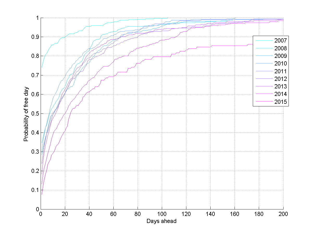
If we slice the data by year, then there seems to be a fairly clear trend towards the planning horizon growing – I have more and more events far into future, and I have more to do. Oh, those halcyon days in 2007 when I presumably just lazed around…

Distance to first day where I have 50%, 75% or 90% chance of being entirely unscheduled.

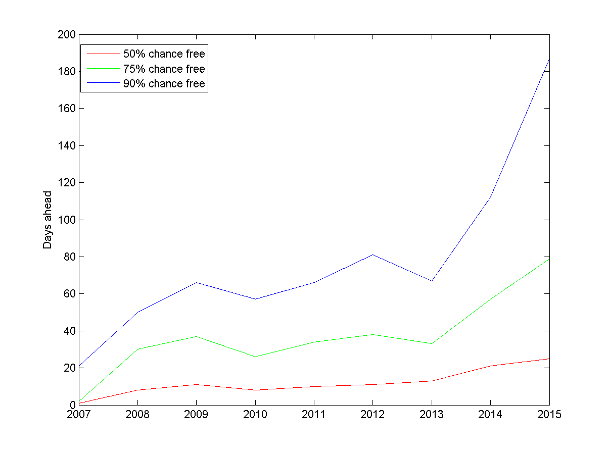
If we plot when I have 50%, 75% and 90% chance of being free, the trend is even clearer. At present you need to ask about three weeks in advance to have a 50% chance of grabbing me, and 187 days in advance to be 90% certain (if you want an entire working week with 50% chance, this is close to where you should go). Back in 2008 the 50% point was about a week and the 90% point 1.5 months ahead. I have become around 3 times busier.

Conclusions

So, I have become busier. This is of course no evidence of getting more done – a lot of events are pointless meetings, and who knows if I am doing anything helpful at the other events. Plus, I might actually be wasting my time doing statistics and blogging instead of working.

But the exercise shows that it is possible to automatically estimate necessary planning horizons. Maybe we should add this to calendar apps to help scheduling: my contact page or virtual secretary might give you an automatically updated estimate of how far ahead you need to schedule things to have a good chance of getting me. It doesn’t have to tell you my detailed schedule (in principle one could do a privacy attack on the schedule by asking for very specific dates and seeing if they were blocked).

We can also use this method to look at levels of busyness across organisations. Who have flexibility in their schedules, who are so overloaded that they cannot be effectively involved in projects? In the past, tasks tended to be simple and the issue was just the amount of time people had. But today we work individually yet as part of teams, and coordination (meetings, seminars, lectures) are the key links: figuring out how to schedule them right is important for effectivity.

If team member $j$ has scheduling rates $\lambda_j(i)$ and they are are uncorrelated (yeah, right), then $Q(t)=\prod_{i=t}^\infty e^{-\sum_j\lambda_j(i)}$ . The most important lesson is that the chance of everybody being able to make it to any given meeting day declines exponentially with the number of people. If the $\lambda_j(i)$ decline exponentially with time (plausible in at least my case) then scheduling a meeting requires the time ahead to be proportional to the number of people involved: double the meeting size, at least double the planning horizon. So if you want nimble meetings, make them tiny.

In the end, I prefer to live by the advice my German teacher Ulla Landvik once gave me, glancing at the school clock: “I see we have 30 seconds left of the lesson. Let’s do this excercise – we have plenty of time!” Time not only flies, it can be stretched too.

Addendum 2015-05-01

Some further explorations.

Days until next completely free day as a function of time. Grey shows data day-by-day, blue averaged over 7 days, green 30 days and red one year.

Owen Cotton-Barratt pointed out that another measure of busyness might be the distance to the next free day. Plotting it shows a very bursty pattern, with noisy peaks. The mean time was about 2-3 days: even though a lot of time the horizon is far away, often an empty day slips through too. It is just that it cannot be relied on.

Histogram of the timing of events by weekday.

Are there periodicities? The most obvious is the weekly dynamics: Thursdays are busiest, weekend least busy. I tend to do scheduling in a roughly similar manner, with Tuesdays as the top scheduling day.

Number of events scheduled per day, plotted across my calendar.

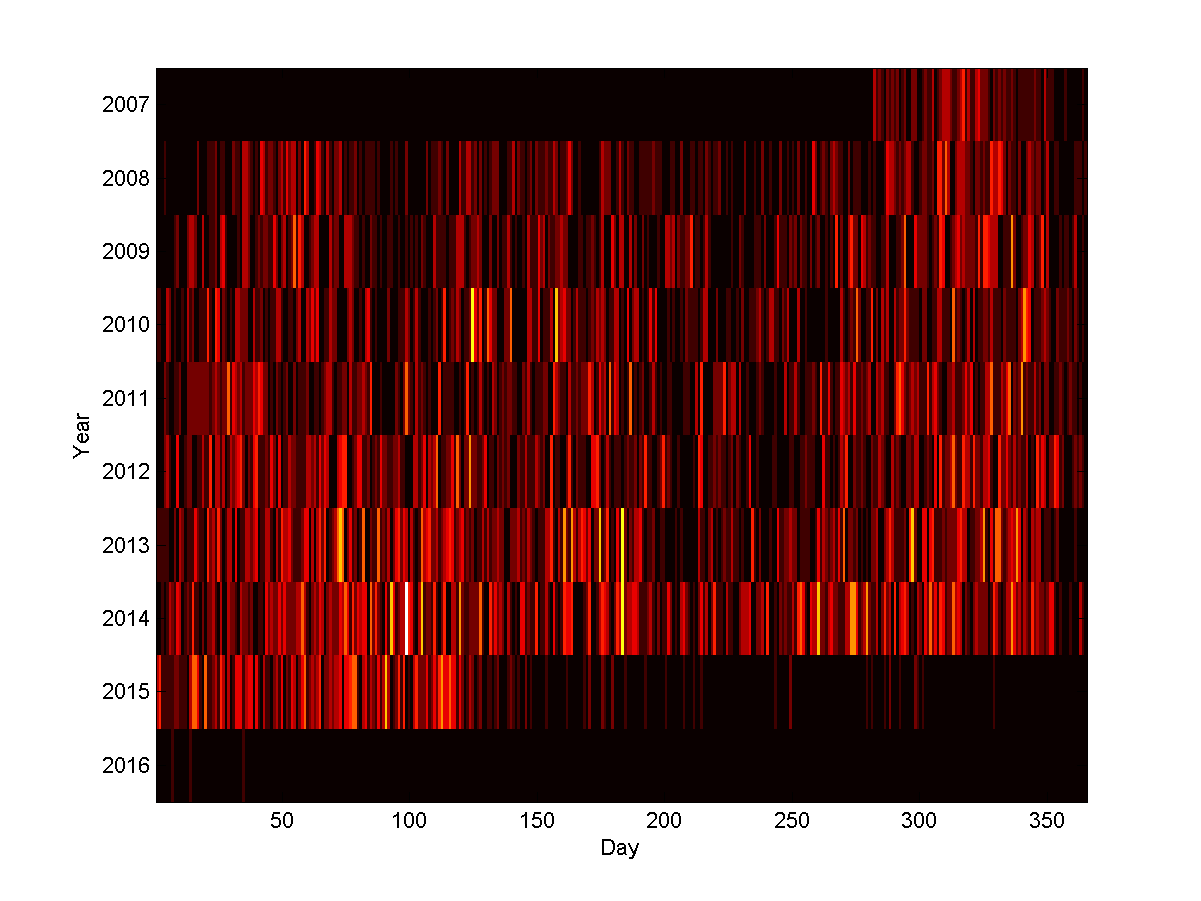
Over the years, plotting the number of events per day (“event intensity”) it is also clear that there is a loose pattern. Back in 2008-2011 one can see a lower rate around day 75 – that is the break between Hilary and Trinity term here in Oxford. There is another trough around day 200-250, the summer break and the time before the Michaelmas term. However, this is getting filled up over time.

Periodogram of event intensity, showing periodicities in my schedule. Note the weekly and yearly peaks.

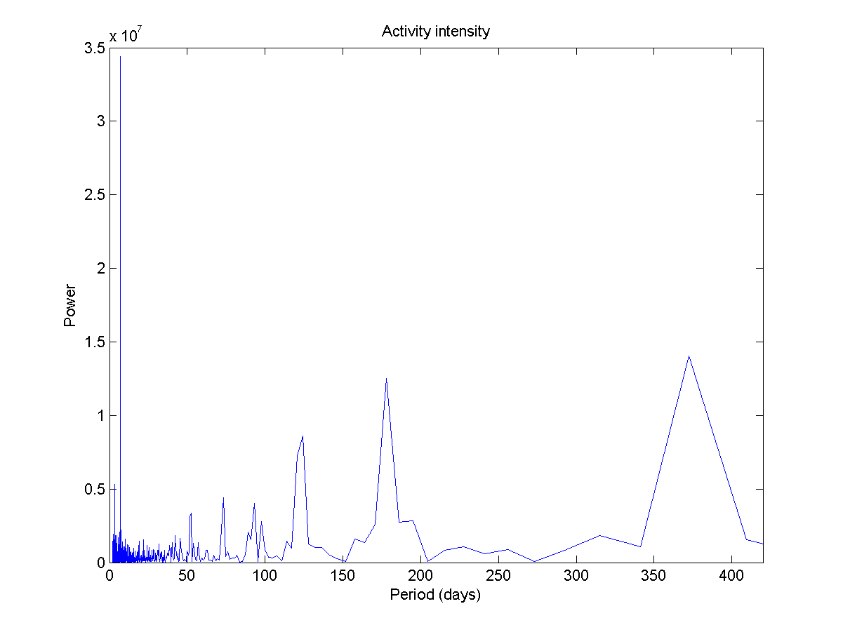
Making a periodogram produces an obvious peak for 7 days, and a loose yearly periodicity. Between them there is a bunch of harmonics. The funny thing is that the week periodicity is very strong but hard to see in the map above.

Crispy embryos

Researchers at Sun Yat-sen University in Guangzhou have edited the germline genome of human embryos (paper). They used the ever more popular CRISPR/Cas9 method to try to modify the gene involved in beta-thalassaemia in non-viable leftover embryos from a fertility clinic.

As usual there is a fair bit of handwringing, especially since there was a recent call for a moratorium on this kind of thing from one set of researchers, and a more liberal (yet cautious) response from another set. As noted by ethicists, many of the ethical concerns are actually somewhat confused.

That germline engineering can have unpredictable consequences for future generations is as true for normal reproduction. More strongly, somebody making the case that (say) race mixing should be hindred because of unknown future effects would be condemned as a racist: we have overarching reasons to allow people live and procreate freely that morally overrule worries about their genetic endowment – even if there actually were genetic issues (as far as I know all branches of the human family are equally interfertile, but this might just be a historical contingency). For a possible future effect to matter morally it needs to be pretty serious and we need to have some real reason to think it is more likely to happen because of the actions we take now. A vague unease or a mere possibility is not enough.

However, the paper actually gives a pretty good argument for why we should not try this method in humans. They found that the efficiency of the repair was about 50%, but more worryingly that there was off-target mutations and that a similar gene was accidentally modified. These are good reasons not to try it. Not unexpected, but very helpful in that we can actually make informed decisions both about whether to use it (clearly not until the problems have been fixed) and what needs to be investigated (how can it be done well? why does it work worse here than advertised?).

The interesting thing with the paper is that the fairly negative results which would reduce interest in human germline changes is anyway hailed as being unethical. It is hard to make this claim stick, unless one buys into the view that germline changes of human embryos is intrinsically bad. The embryos could not develop into persons and would have been discarded from the fertility clinic, so there was no possible future person being harmed (if one thinks fertilized but non-viable embryos deserve moral protection one has other big problems). The main fear seems to be that if the technology is demonstrated many others will follow, but an early negative result would seem to reduce this slippery slope argument.

I think the real reason people think there is an ethical problem is the association of germline engineering with “designer babies”, and the conditioning that designer babies are wrong. But they can’t be wrong for no reason: there has to be an ethics argument for their badness. There is no shortage of such arguments in the literature, ranging from ideas of the natural order, human dignity, accepting the given, the importance of an open-ended life to issues of equality, just to mention a few. But none of these are widely accepted as slam-dunk arguments that conclusively show designer babies are wrong: each of them also have vigorous criticisms. One can believe one or more of them to be true, but it would be rather premature to claim that settles the debate. And even then, most of these designer baby arguments are irrelevant for the case at hand.

All in all, it was a useful result that probably will reduce both risky and pointless research and focus on what matters. I think that makes it quite ethical.

The end of the worlds

George Dvorsky has a piece on Io9 about ways we could wreck the solar system, where he cites me in a few places. This is mostly for fun, but I think it links to an important existential risk issue: what conceivable threats have big enough spatial reach to threaten a interplanetary or even star-faring civilization?

This matters, since most existential risks we worry about today (like nuclear war, bioweapons, global ecological/societal crashes) only affect one planet. But if existential risk is the answer to the Fermi question, then the peril has to strike reliably. If it is one of the local ones it has to strike early: a multi-planet civilization is largely immune to the local risks. It will not just be distributed, but it will almost by necessity have fairly self-sufficient habitats that could act as seeds for a new civilization if they survive. Since it is entirely conceivable that we could have invented rockets and spaceflight long before discovering anything odd about uranium or how genetics work it seems unlikely that any of these local risks are “it”. That means that the risks have to be spatially bigger (or, of course, that xrisk is not the answer to the Fermi question).

Of the risks mentioned by George physics disasters are intriguing, since they might irradiate solar systems efficiently. But the reliability of them being triggered before interstellar spread seems problematic. Stellar engineering, stellification and orbit manipulation may be issues, but they hardly happen early – lots of time to escape. Warp drives and wormholes are also likely late activities, and do not seem to be reliable as extinctors. These are all still relatively localized: while able to irradiate a largish volume, they are not fine-tuned to cause damage and does not follow fleeing people. Dangers from self-replicating or self-improving machines seems to be a plausible, spatially unbound risk that could pursue (but also problematic for the Fermi question since now the machines are the aliens). Attracting malevolent aliens may actually be a relevant risk: assuming von Neumann probes one can set up global warning systems or “police probes” that maintain whatever rules the original programmers desire, and it is not too hard to imagine ruthless or uncaring systems that could enforce the great silence. Since early civilizations have the chance to spread to enormous volumes given a certain level of technology, this might matter more than one might a priori believe.

So, in the end, it seems that anything releasing a dangerous energy effect will only affect a fixed volume. If it has energy $E$ and one can survive it below a deposited energy $e$ , if it just radiates in all directions the safe range is $r = \sqrt{E/4 \pi e} \propto \sqrt{E}$ – one needs to get into supernova ranges to sterilize interstellar volumes. If it is directional the range goes up, but smaller volumes are affected: if a fraction $f$ of the sky is affected, the range increases as $\propto \sqrt{1/f}$ but the total volume affected scales as $\propto f\sqrt{1/f}=\sqrt{f}$ .

Self-sustaining effects are worse, but they need to cross space: if their space range is smaller than interplanetary distances they may destroy a planet but not anything more. For example, a black hole merely absorbs a planet or star (releasing a nasty energy blast) but does not continue sucking up stuff. Vacuum decay on the other hand has indefinite range in space and moves at lightspeed. Accidental self-replication is unlikely to be spaceworthy unless is starts among space-moving machinery; here deliberate design is a more serious problem.

The speed of threat spread also matters. If it is fast enough no escape is possible. However, many of the replicating threats will have sublight speed and could hence be escaped by sufficiently paranoid aliens. The issue here is if lightweight and hence faster replicators can always outrun larger aliens; given the accelerating expansion of the universe it might be possible to outrun them by being early enough, but our calculations do suggest that the margins look very slim.

The more information you have about a target, the better you can in general harm it. If you have no information, merely randomizing it with enough energy/entropy is the only option (and if you have no information of where it is, you need to radiate in all directions). As you learn more, you can focus resources to make more harm per unit expended, up to the extreme limits of solving the optimization problem of finding the informational/environmental inputs that cause desired harm (=hacking). This suggests that mindless threats will nearly always have shorter range and smaller harms than threats designed by (or constituted by) intelligent minds.

In the end, the most likely type of actual civilization-ending threat for an interplanetary civilization looks like it needs to be self-replicating/self-sustaining, able to spread through space, and have at least a tropism towards escaping entities. The smarter, the more effective it can be. This includes both nasty AI and replicators, but also predecessor civilizations that have infrastructure in place. Civilizations cannot be expected to reliably do foolish things with planetary orbits or risky physics.

[Addendum: Charles Stross has written an interesting essay on the risk of griefers as a threat explanation. ]

[Addendum II: Robin Hanson has a response to the rest of us, where he outlines another nasty scenario. ]

Andart II

Part of Anders' Exoself

Month: April 2015