I have a glass cube on my office windowsill containing a slice of a Calabi-Yau manifold, one of Bathsheba Grossman’s wonderful creations. It is an intricate, self-intersecting surface with lots of unexpected symmetries. A visiting friend got me into trying to make my own version of the surface.
First, what is the equation for it? Grossman-Hanson’s explanation is somewhat involved, but basically what we are seeing is a 2D slice through a 6-dimensional manifold in a projective space expressed as the 4D manifold 
=e^{2\pi i k_1 / n}\cosh(\theta+\xi i)^{2/n}")
=e^{2 \pi i k_2 / n}\sinh(\theta+\xi i)^{2/n}/i")
where the k’s run through ")

,\Re(z_2),\cos(\alpha)\Im(z_1)+\sin(\alpha)\Im(z_2))")
where 
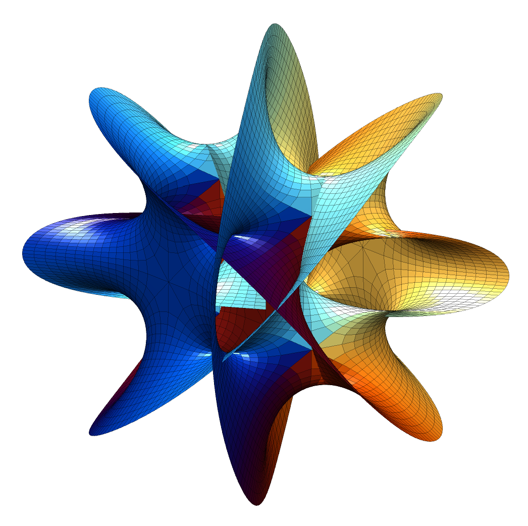
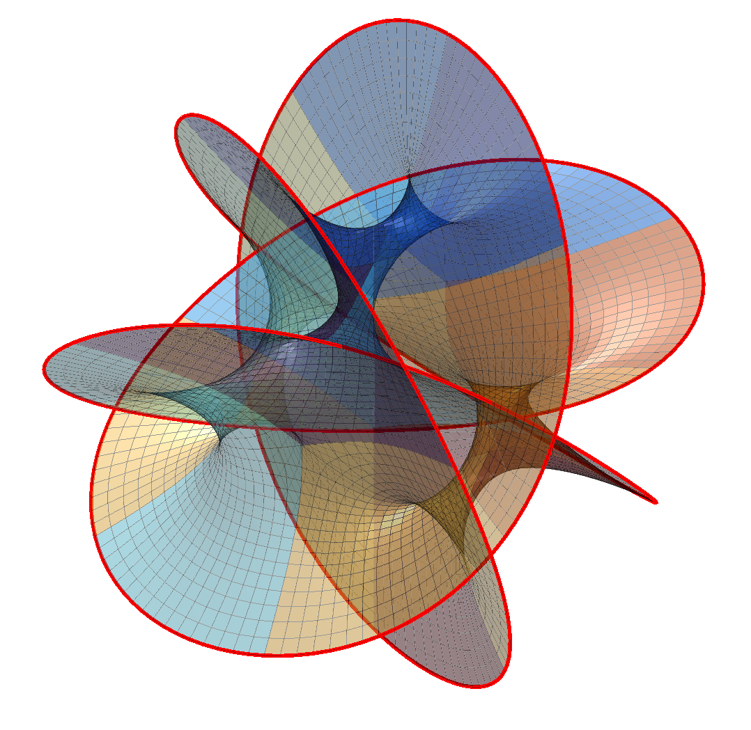
The result is pretty nifty. It is tricky to see how it hangs together in 2D; rotating it in 3D helps a bit. It is composed of 16 identical patches:
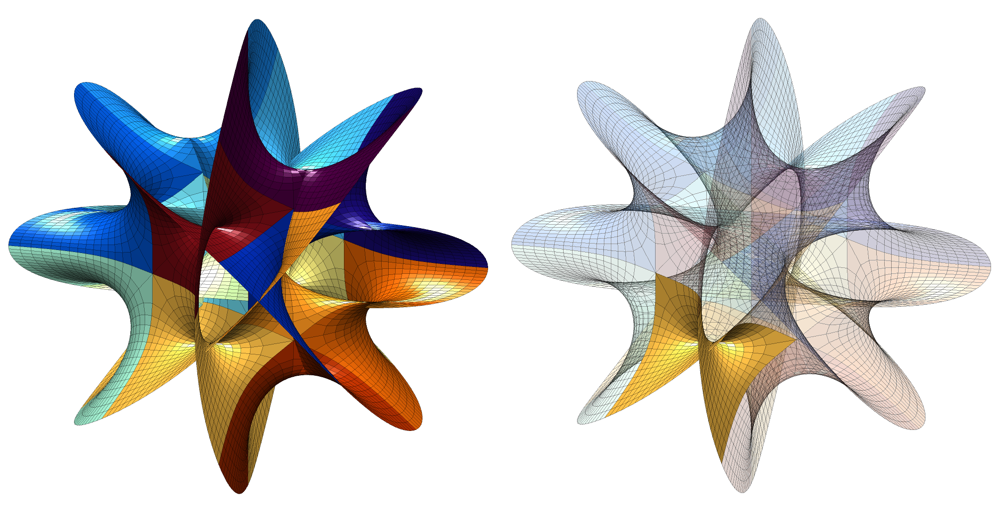
The boundary of the patches meet other patches except along two open borders (corresponding to large or small values of 
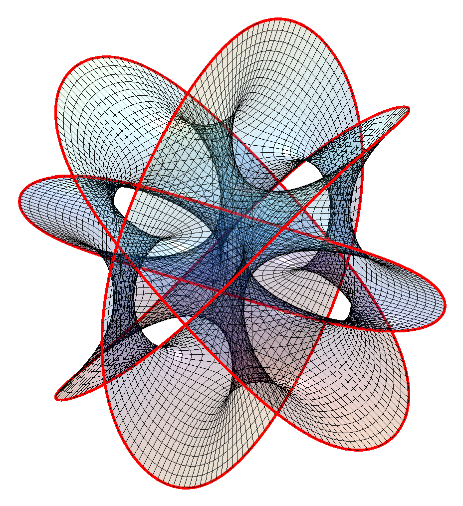
A surface bounded by a knot or a link is called a Seifert surface. While these surfaces look a lot like minimal surfaces they are not exactly minimal when I estimate the mean curvature (it should be exactly zero); while this could be because of lack of numerical precision I think it is real: while minimal surfaces are Ricci-flat, the converse is not necessarily true.
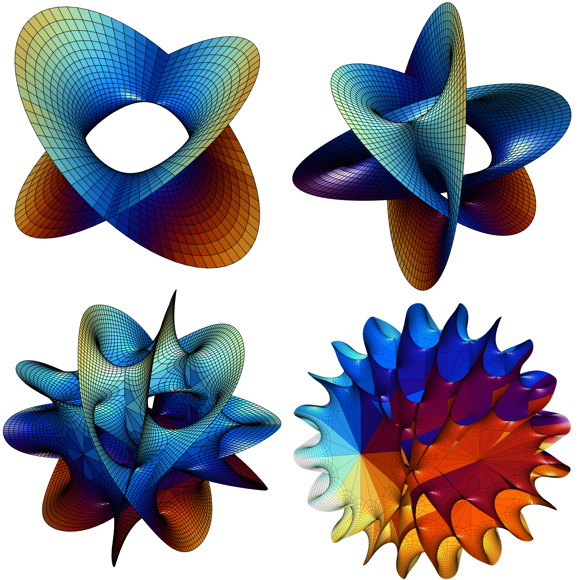
Changing N produces other surfaces. N=2 is basically a catenoid (tilted and self-intersecting). As N increases it becomes more like a barrel or a pufferfish, with one direction dominated by circular saddle regions, one showing a meshwork of spaces reminiscent of spacefilling minimal surfaces, and one a lot of overlapping “barbs”.
Note that just like for minimal surfaces one can multiply 

Hanson also notes that by changing the formula to 
=e^{2\pi i k_1 / n_1}\cosh(\theta+\xi i)^{2/n_1}")
=e^{2 \pi i k_2 / n_2}\sinh(\theta+\xi i)^{2/n_2}/i")
Appendix: Matlab code
%% Initialization

edge=0; % Mark edge?

coloring=1; % Patch coloring type

n=4;

s=0.1; % Gridsize

alp=1; ca=cos(alp); sa=sin(alp); % Projection

[theta,xi]=meshgrid(-1.5:s:1.5,1*(pi/2)*(0:1:16)/16);

z=theta+xi*i;

% Color scheme

tt=2*pi*(1:200)'/200; co=.5+.5*[cos(tt) cos(tt+1) cos(tt+2)];

colormap(co)

%% Plot

clf

hold on

for k1=0:(n-1)

for k2=0:(n-1)

z1=exp(k1*2*pi*i/n)*cosh(z).^(2/n);

z2=exp(k2*2*pi*i/n)*(1/i)*sinh(z).^(2/n);

X=real(z1);

Y=real(z2);

Z=ca*imag(z1)+sa*imag(z2);

if (coloring==0)

surf(X,Y,Z);

else

switch (coloring)

case 1

C=z1*0+(k1+k2*n); % Color by patch

case 2

C=abs(z1);

case 3

C=theta;

case 4

C=xi;

case 5

C=angle(z1);

case 6

C=z1*0+1;

end

h=surf(X,Y,Z,C);

set(h,'EdgeAlpha',0.4)

end

if (edge>0)

plot3(X(:,end),Y(:,end),Z(:,end),'r','LineWidth',2)

plot3(X(:,1),Y(:,1),Z(:,1),'r','LineWidth',2)

end

end

end

view([2 3 1])

camlight

h=camlight('left');

set(h,'Color',[1 1 1]*.5)

axis equal

axis vis3d

axis off