Bring back the dead

I recently posted a brief essay on The Conversation about the ethics of trying to regenerate the brains of brain dead patients (earlier version posted later on Practical Ethics). Tonight I am giving interviews on BBC World radio about it.

The quick of it is that it will mess with our definitions of who happens to be dead, but that is mostly a matter of sorting out practice and definitions, and that it is somewhat questionable who is benefiting: the original patient is unlikely to recover, but we might get a moral patient we need to care for even if they are not a person, or even a different person (or most likely, just generally useful medical data but no surviving patient at all). The problem is that partial success might be worse than no success. But the only way of knowing is to try.

The Drake equation and correlations

I have been working on the Fermi paradox for a while, and in particular the mathematical structure of the Drake equation. While it looks innocent, it has some surprising issues.

$N\approx N_* f_p n_e f_l f_i f_c L$

One area I have not seen much addressed is the independence of terms. To a first approximation they were made up to be independent: the fraction of life-bearing Earth-like planets is presumably determined by a very different process than the fraction of planets that are Earth-like, and these factors should have little to do with the longevity of civilizations. But as Häggström and Verendel showed, even a bit of correlation can cause trouble.

If different factors in the Drake equation vary spatially or temporally, we should expect potential clustering of civilizations: the average density may be low, but in areas where the parameters have larger values there would be a higher density of civilizations. A low $N$ may not be the whole story. Hence figuring out the typical size of patches (i.e. the autocorrelation distance) may tell us something relevant.

Astrophysical correlations

There is a sometimes overlooked spatial correlation in the first terms. In the orthodox formulation we are talking about earth-like planets orbiting stars with planets, which form at some rate in the Milky Way. This means that civilizations must be located in places where there are stars (galaxies), and not anywhere else. The rare earth crowd also argues that there is a spatial structure that makes earth-like worlds exist within a ring-shaped region in the galaxy. This implies an autocorrelation on the order of (tens of) kiloparsecs.

Even if we want to get away from planetocentrism there will be inhomogeneity. The warm intergalactic plasma contains 0.04 of the total mass of the universe, or 85% of the non-dark stuff. Planets account for just 0.00002%, and terrestrials obviously far less. Since condensed things like planets, stars or even galaxy cluster plasma is distributed in a inhomogeneous manner, unless the other factors in the Drake equation produce typical distances between civilizations beyond the End of Greatness scale of hundreds of megaparsec, we should expect a spatially correlated structure of intelligent life following galaxies, clusters and filiaments.

A tangent: different kinds of matter plausibly have different likelihood of originating life. Note that this has an interesting implication: if the probability of life emerging in something like the intergalactic plasma is non-zero, it has to be more than a hundred thousand times smaller than the probability per unit mass of planets, or the universe would be dominated by gas-creatures (and we would be unlikely observers, unless gas-life was unlikely to generate intelligence). Similarly life must be more than 2,000 times more likely on planets than stars (per unit of mass), or we should expect ourselves to be star-dwellers. Our planetary existence does give us some reason to think life or intelligence in the more common substrates (plasma, degenerate matter, neutronium) is significantly less likely than molecular matter.

Biological correlations

One way of inducing correlations in the $f_l$ factor is panspermia. If life originates at some low rate per unit volume of space (we will now assume a spatially homogeneous universe in terms of places life can originate) and then diffuses from a nucleation site, then intelligence will show up in spatially correlated locations.

It is not clear how much panspermia could be going on, or if all kinds of life do it. A simple model is that panspermias emerge at a density $\rho$ and grow to radius $r$ . The rate of intelligence emergence outside panspermias is set to 1 per unit volume (this sets a space scale), and inside a panspermia (since there is more life) it will be $A>1$ per unit volume. The probability that a given point will be outside a panspermia is

$P_{outside} = e^{-(4\pi/3) r^3 \rho}$ .

The fraction of civilizations finding themselves outside panspermias will be

$F_{outside} = \frac{P_{outside}}{P_{outside}+A(1-P_{outside})} = \frac{1}{1+A(e^{(4 \pi/3)r^3 \rho}-1)}$ .

As A increases, vastly more observers will be in panspermias. If we think it is large, we should expect to be in a panspermia unless we think the panspermia efficiency (and hence r) is very small. Loosely, the transition from going from 1% to 99% probability takes one order of magnitude change in r, three orders of magnitude in $\rho$ and four in A: given that these parameters can a priori range over many, many orders of magnitude, we should not expect to be in the mixed region where there are comparable numbers of observers inside panspermias and outside. It is more likely all or nothing.

There is another relevant distance beside $r$ , the expected distance to the next civilization. This is $d \approx 0.55/\sqrt[3]{\lambda}$ where $\lambda$ is the density of civilizations. For the outside panspermia case this is $d_{outside}=0.55$ , while inside it is $d_{inside}=0.55/\sqrt[3]{A}$ . Note that these distances are not dependent on the panspermia sizes, since they come from an independent process (emergence of intelligence given a life-bearing planet rather than how well life spreads from system to system).

If $r<d_{inside}$ then there will be no panspermia-induced correlation between civilization locations, since there is less than one civilization per panspermia. For $d_{inside} < r < d_{outside}$ there will be clustering with a typical autocorrelation distance corresponding to the panspermia size. For even larger panspermias they tend to dominate space (if $\rho$ is not very small) and there is no spatial structure any more.

So if panspermias have sizes in a certain range, $0.55/\sqrt[3]{A}<r<0.55$ , the actual distance to the nearest neighbour will be smaller than what one would have predicted from the average values of the parameters of the drake equation.

Nearest neighbor distance for civilizations in a model with spherical panspermias and corresponding randomly resampled distribution. — Nearest neighbour distance for civilizations in a model with spherical panspermias and corresponding randomly re-sampled distribution.

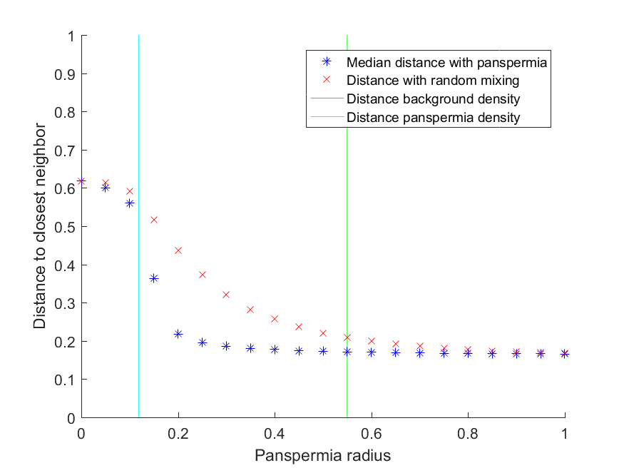
Running a Monte Carlo simulation shows this effect. Here I use 10,000 possible life sites in a cubical volume, and $\rho=1$ – the number of panspermias will be Poisson(1) distributed. The background rate of civilizations appearing is 1/10,000, but in panspermias it is 1/100. As I make panspermias larger civilizations become more common and the median distance from a civilization to the next closest civilization falls (blue stars). If I re-sample so the number of civilizations are the same but their locations are uncorrelated I get the red crosses: the distances decline, but they can be more than a factor of 2 larger.

Technological correlations

The technological terms $f_c$ and $L$ can also show spatial patterns, if civilizations spread out from their origin.

The basic colonization argument by Hart and Tipler assumes a civilization will quickly spread out to fill the galaxy; at this point $N\approx 10^{10}$ if we count inhabited systems. If we include intergalactic colonization, then in due time, everything out to a radius of reachability on the order of 4 gigaparsec (for near c probes) and 1.24 gigaparsec (for 50% c probes). Within this domain it is plausible that the civilization could maintain whatever spatio-temporal correlations it wishes, from perfect homogeneity over the zoo hypothesis to arbitrary complexity. However, the reachability limit is due to physics and do impose a pretty powerful limit: any correlation in the Drake equation due to a cause at some point in space-time will be smaller than the reachability horizon (as measured in comoving coordinates) for that point.

Total colonization is still compatible with an empty galaxy if $L$ is short enough. Galaxies could be dominated by a sequence of “empires” that disappear after some time, and if the product between empire emergence rate $\lambda$ and $L$ is small enough most eras will be empty.

A related model is Brin’s resource exhaustion model, where civilizations spread at some velocity but also deplete their environment at some (random rate). The result is a spreading shell with an empty interior. This has some similarities to Hanson’s “burning the cosmic commons scenario”, although Brin is mostly thinking in terms of planetary ecology and Hanson in terms of any available resources: the Hanson scenario may be a single-shot situation. In Brin’s model “nursery worlds” eventually recover and may produce another wave. The width of the wave is proportional to $Lv$ where $v$ is the expansion speed; if there is a recovery parameter $R$ corresponding to the time before new waves can emerge we should hence expect spatial correlation length of order $(L+R)v$ . For light-speed expansion and a megayear recovery (typical ecology and fast evolutionary timescale) we would get a length of a million light-years.

Another approach is the percolation theory inspired models first originated by Landis. Here civilizations spread short distances, and “barren” offshoots that do not colonize form a random “bark” around the network of colonization (or civilizations are limited to flights shorter than some distance). If the percolation parameter $p$ is low, civilizations will only spread to a small nearby region. When it increases larger and larger networks are colonized (forming a fractal structure), until a critical parameter value $p_c$ where the network explodes and reaches nearly anywhere. However, even above this transition there are voids of uncolonized worlds. The correlation length famously scales as $\xi \propto|p-p_c|^\nu$ , where $\nu \approx -0.89$ for this case. The probability of a random site belonging to the infinite cluster for $p>p_c$ scales as $P(p) \propto |p-p_c|^\beta$ ( $\beta \approx 0.472$ ) and the mean cluster size (excluding the infinite cluster) scales as $\propto |p-p_c|^\gamma$ ( $\gamma \approx -1.725$ ).

So in this group of models, if the probability of a site producing a civilization is $\lambda$ the probability of encountering another civilization in one’s cluster is

$Q(p) = 1-(1-\lambda)^{N|p-p_c|^\gamma}$

for $p<p_c$ . Above the threshold it is essentially 1; there is a small probability $1-P(p)$ of being inside a small cluster, but it tends to be minuscule. Given the silence in the sky, were a percolation model the situation we should conclude either an extremely low $\lambda$ or a low $p$ .

Temporal correlations

Another way the Drake equation can become misleading is if the parameters are time varying. Most obviously, the star formation rate has changed over time. The metallicity of stars have changed, and we should expect any galactic life zones to shift due to this.

One interesting model due to James Annis and Milan Cirkovic is that the rate of gamma ray bursts and other energetic disasters made complex life unlikely in the past, but now the rate has declined enough that it can start the climb towards intelligence – and it was synchronized by this shared background. Such disasters can also produce spatial coherency, although it is very noisy.

In my opinion the most important temporal issue is inherent in the Drake equation itself. It assumes a steady state! At the left we get new stars arriving at a rate $N_*$ , and at the right the rate gets multiplied by the longevity term for civilizations $L$ , producing a dimensionless number. Technically we can plug in a trillion years for the longevity term and get something that looks like a real estimate of a teeming galaxy, but this actually breaks the model assumptions. If civilizations survived for trillions of years, the number of civilizations would currently be increasing linearly (from zero at the time of the formation of the galaxy) – none would have gone extinct yet. Hence we can know that in order to use the unmodified Drake equation $L$ has to be $< 10^{10}$ years.

Making a temporal Drake equation is not impossible. A simple variant would be something like

$\frac{dN(t)}{dt}=N_*(t)f_p(t)n_e(t)f_l(t)f_i(t)f_c(t)-(1/L)N$

where the first term is just the factors of the vanilla equation regarded as time-varying functions and the second term a decay corresponding to civilizations dropping out at a rate of 1/L (this assumes exponentially distributed survival, a potentially doubtful assumption). The steady state corresponds to the standard Drake level, and is approached with a time constant of 1/L. One nice thing with this equation is that given a particular civilization birth rate $\beta(t)$ corresponding to the first term, we get an expression for the current state:

$N(t_{now}) = \int_{t_{bigbang}}^{t_{now}} \beta(t) e^{-(1/L) (t_{now}-t)} dt$ .

Note how any spike in $\beta(t)$ gets smoothed by the exponential, which sets the temporal correlation length.

If we want to do things even more carefully, we can have several coupled equations corresponding to star formation, planet formation, life formation, biosphere survival, and intelligence emergence. However, at this point we will likely want to make a proper “demographic” model that assumes stars, biospheres and civilization have particular lifetimes rather than random disappearance. At this point it becomes possible to include civilizations with different L, like Sagan’s proposal that the majority of civilizations have short L but some have very long futures.

The overall effect is still a set of correlation timescales set by astrophysics (star and planet formation rates), biology (life emergence and evolution timescales, possibly the appearance of panspermias), and civilization timescales (emergence, spread and decay). The overall effect is dominated by the slowest timescale (presumably star formation or very long-lasting civilizations).

Conclusions

Overall, the independence of the terms of the Drake equation is likely fairly strong. However, there are relevant size scales to consider.

Over multiple gigaparsec scales there can not be any correlations, not even artificially induced ones, because of limitations due to the expansion of the universe (unless there are super-early or FTL civilizations).
Over hundreds of megaparsec scales the universe is fairly uniform, so any natural influences will be randomized beyond this scale.
Colonization waves in Brin’s model could have scales on the galactic cluster scale, but this is somewhat parameter dependent.
The nearest civilization can be expected around $d \approx 0.55 [N_* f_p n_e f_l f_i f_c L / V]^{-1/3}$ , where $V$ is the galactic volume. If we are considering parameters such that the number of civilizations per galaxy are low V needs to be increased and the density will go down significantly (by a factor of about 100), leading to a modest jump in expected distance.
Panspermias, if they exist, will have an upper extent limited by escape from galaxies – they will tend to have galactic scales or smaller. The same is true for galactic habitable zones if they exist. Percolation colonization models are limited to galaxies (or even dense parts of galaxies) and would hence have scales in the kiloparsec range.
“Scars” due to gamma ray bursts and other energetic events are below kiloparsecs.
The lower limit of panspermias are due to $d$ being smaller than the panspermia, presumably at least in the parsec range. This is also the scale of close clusters of stars in percolation models.
Time-wise, the temporal correlation length is likely on the gigayear timescale, dominated by stellar processes or advanced civilization survival. The exception may be colonization waves modifying conditions radically.

In the end, none of these factors appear to cause massive correlations in the Drake equation. Personally, I would guess the most likely cause of an observed strong correlation between different terms would be artificial: a space-faring civilization changing the universe in some way (seeding life, wiping out competitors, converting it to something better…)

Aristotle on trolling

A new translation of Aristotle’s classic “On trolling” by Rachel Barney! (Open Access)

That trolling is a shameful thing, and that no one of sense would accept to be called ‘troll’, all are agreed; but what trolling is, and how many its species are, and whether there is an excellence of the troll, is unclear. And indeed trolling is said in many ways; for some call ‘troll’ anyone who is abusive on the internet, but this is only the disagreeable person, or in newspaper comments the angry old man. And the one who disagrees loudly on the blog on each occasion is a lover of controversy, or an attention-seeker. And none of these is the troll, or perhaps some are of a mixed type; for there is no art in what they do. (Whether it is possible to troll one’s own blog is unclear; for the one who poses divisive questions seems only to seek controversy, and to do so openly; and this is not trolling but rather a kind of clickbait.)

Aristotle’s definition is quite useful:

The troll in the proper sense is one who speaks to a community and as being part of the community; only he is not part of it, but opposed. And the community has some good in common, and this the troll must know, and what things promote and destroy it: for he seeks to destroy.

He then goes on analysing the knowledge requirements of trolling, the techniques, the types or motivations of trolls, the difference between a gadfly like Socrates and a troll, and what communities are vulnerable to trolls. All in a mere two pages.

(If only the medieval copyists had saved his other writings on the Athenian Internet! But the crash and split of Alexander the Great’s social media empire destroyed many of them before that era.)

The text reminds me of another must-read classic, Harry Frankfurt’s “On Bullshit”. There Frankfurt analyses the nature of bullshitting. His point is that normal deception cares about the truth: it aims to keep someone from learning it. But somebody producing bullshit does not care about the truth or falsity of the statements made, merely that they fit some manipulative, social or even time-filling aim.

It is just this lack of connection to a concern with truth – this indifference to how things really are – that I regard as of the essence of bullshit.

It is pernicious, since it fills our social and epistemic arena with dodgy statements whose value is uncorrelated to reality, and the bullshitters gain from the discourse being more about the quality (or the sincerity) of bullshitting than any actual content.

Both of these essays are worth reading in this era of the Trump candidacy and Dugin’s Eurasianism. Know your epistemic enemies.

Review of “Here be Dragons” by Olle Häggström

By Anders Sandberg, Future of Humanity Institute, Oxford Martin School, University of Oxford

Thinking of the future is often done as entertainment. A surprising number of serious-sounding predictions, claims and prophecies are made with apparently little interest in taking them seriously, as evidenced by how little they actually change behaviour or how rarely originators are held responsible for bad predictions. Rather, they are stories about our present moods and interests projected onto the screen of the future. Yet the future matters immensely: it is where we are going to spend the rest of our lives. As well as where all future generations will live – unless something goes badly wrong.

Olle Häggström’s book is very much a plea for taking the future seriously, and especially for taking exploring the future seriously. As he notes, there are good reasons to believe that many technologies under development will have enormous positive effects… and also good reasons to suspect that some of them will be tremendously risky. It makes sense to think about how we ought to go about avoiding the risks while still reaching the promise.

Current research policy is often directed mostly towards high quality research rather than research likely to make a great difference in the long run. Short term impact may be rewarded, but often naively: when UK research funding agencies introduced impact evaluation a few years back, their representatives visiting Oxford did not respond to the question on whether impact had to be positive. Yet, as Häggström argues, obviously the positive or negative impact of research must matter! A high quality investigation into improved doomsday weapons should not be pursued. Investigating the positive or negative implications of future research and technology has high value, even if it is difficult and uncertain.

Inspired by James Martin’s The Meaning of the 21^st Century this book is an attempt to make a broad map sketch of parts of the future that matters, especially the uncertain corners where we have reason to think dangerous dragons lurk. It aims more at scope than the detail of many of the covered topics, making it an excellent introduction and pointer towards the primary research.

One obvious area is climate change, not just in terms of its direct (and widely recognized risks) but the new challenges posed by geoengineering. Geoengineering may both be tempting to some nations and possible to perform unilaterally, yet there are a host of ethical, political, environmental and technical risks linked to it. It also touches on how far outside the box we should search for solutions: to many geoengineering is already too far, but other proposals such as human engineering (making us more eco-friendly) go much further. When dealing with important challenges, how do we allocate our intellectual resources?

Other areas Häggström reviews include human enhancement, artificial intelligence, and nanotechnology. In each of these areas tremendously promising possibilities – that would merit a strong research push towards them – are intermixed with different kinds of serious risks. But the real challenge may be that we do not yet have the epistemic tools to analyse these risks well. Many debates in these areas contain otherwise very intelligent and knowledgeable people making overconfident and demonstrably erroneous claims. One can also argue that it is not possible to scientifically investigate future technology. Häggström disagrees with this: one can analyse it based on currently known facts and using careful probabilistic reasoning to handle the uncertainty. That results are uncertain does not mean they are useless for making decisions.

He demonstrates this by analysing existential risks, scenarios for the long term future humanity and what the “Fermi paradox” may tell us about our chances. There is an interesting interplay between uncertainty and existential risk. Since our species can end only once, traditional frequentist approaches run into trouble Bayesian methods do not. Yet reasoning about events that are unprecedented also makes our arguments terribly sensitive to prior assumptions, and many forms of argument are more fragile than they first look. Intellectual humility is necessary for thinking about audacious things.

In the end, this book is as much a map of relevant areas of philosophy and mathematics containing tools for exploring the future, as it is a direct map of future technologies. One can read it purely as an attempt to sketch where there may be dragons in the future landscape, but also as an attempt at explaining how to go about sketching the landscape. If more people were to attempt that, I am confident that we would fence in the dragons better and direct our policies towards more dragon-free regions. That is a possibility worth taking very seriously.

[Conflict of interest: several of my papers are discussed in the book, both critically and positively.]

Simple instability

As a side effect of a chat about dynamical systems models of metabolic syndrome, I came up with the following nice little toy model showing two kinds of instability: instability because of insufficient dampening, and instability because of too slow dampening.

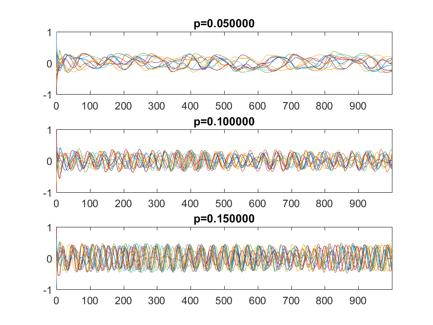
$x'(t) = Ax(t)/N - px(t-\tau) -x(t)^3$

Where $x$ is a N-dimensional vector, A is a $N \times N$ matrix with Gaussian random numbers, and $p \geq 0, \tau \geq 0$ constants. The last term should strictly speaking be written as $||x(t)||^2 x(t)$ but I am lazy.

The first term causes chaos, as we will see below. The 1/N factor is just to compensate for the N terms. The middle term represents dampening trying to force the system to the origin, but acting with a delay $\tau$ . The final term keeps the dynamics bounded: as $||x||$ becomes large this term will dominate and bring back the trajectory to the vicinity of the origin. However, it is a soft spring that has little effect close to the origin.

Chaos

Let us consider the obvious fixed point $x=0$ . Is it stable? If we calculate the Jacobian matrix there it becomes $J = A/N - pI$ . First, consider the case where $p=0$ . The eigenvalues of J will be the ones of a random Gaussian matrix with no symmetry conditions. If it had been symmetric, then Wigner’s semicircle rule implies that they would tend to be distributed as $P(\lambda)=(2/\pi)\sqrt{1-\lambda^2}$ as $N \rightarrow \infty$ . However, it turns out that this is true for the non-symmetric Gaussian case too. (and might be true for any i.i.d. random numbers). This means that about half of them will have a positive real part, and that implies that the fixed point is unstable: for $p=0$ the system will be orbiting the origin in some fashion, and generically this means a chaotic attractor.

Stability

If $p$ grows the diagonal elements of J will become more and more negative. If they are really negative then we essentially have a matrix with a negative diagonal and some tiny off-diagonal terms: the eigenvalues will almost be the diagonal ones, and they are all negative. The origin is a stable attractive fixed point in this limit.

Distribution of eigenvalues of A-fI as the restoring forcing becomes stronger. — Distribution of real part of the eigenvalues of J=A-pI as the restoring forcing becomes stronger. At p=0.1 all eigenvalues have negative real part.

In between, if we plot the eigenvalues as a function of $p$ , we see that the semicircle just linearly moves towards the negative side and when all of it passes over, we shift from the chaotic dynamics to the fixed point. Exactly when this happens depends on the particular A we are looking at and its largest eigenvalue (which is distributed as the Tracy-Widom distribution), but it is generally pretty sharp for large N.

Delay

But what if $\tau$ becomes large? In this case the force moving the trajectory towards the origin will no longer be based on where it is right now, but on where it was $\tau$ seconds earlier. If $p$ is small, then this is just minor noise/bias (and the dynamics is chaotic anyway). If it is large, then the trajectory will be pushed in some essentially random direction: we get instability again.

Plot of the norm |x(t)| for some late value of t as a function of the power and delay. The dark blue square is convergence to zero, the left curved surface is chaotic motion, and the right/back surface is the delay-driven oscillations. — Plot of the average norm |x(t)| for some late value of t as a function of the power and delay. The dark blue square is convergence to zero, the left curved surface is chaotic motion, and the right/back surface is the delay-driven oscillations.

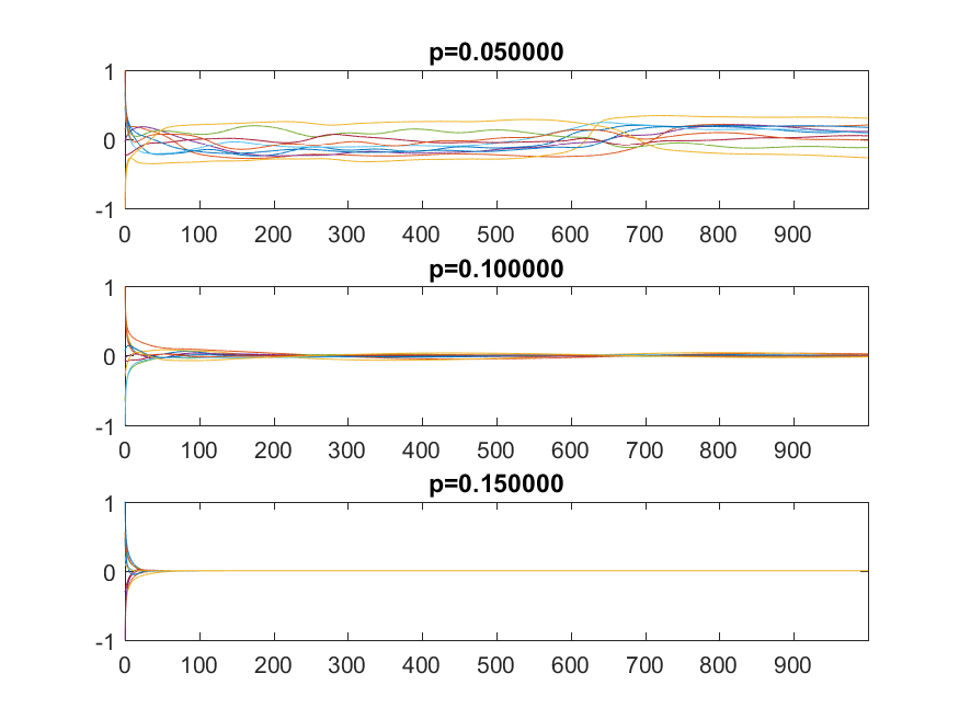
A (very slightly) more stringent way of thinking of it is to plug in $x_j(t)=c_j e^{i\lambda_j t}$ into the equation. To simplify, let’s throw away the cubic term since we want to look at behavior close to zero, and let’s use a coordinate system where the matrix is a diagonal matrix $\Lambda$ . Then for $p=0$ we get $\lambda_j = \Lambda_j$ , that is, the origin is a fixed point that repels or attracts trajectories depending on its eigenvalues (and we know from above that we can be pretty confident some are positive, so it is unstable overall). For $p>0$ we get $\lambda_j + pe^{-i\lambda_j \tau} = \Lambda_j$ . 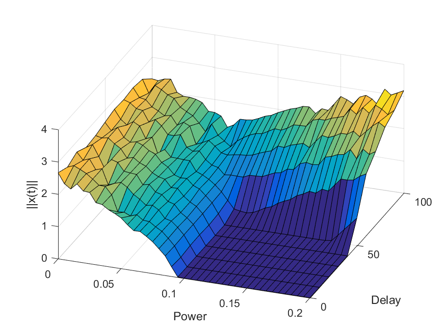Taylor expansion to the first order and rearranging gives us $\lambda_j \approx(\Lambda_j - p)/(1 - i p \tau)$ . The numerator means that as $p$ grows, each eigenvalue will eventually get a negative real part: that particular direction of dynamics becomes stable and attracted to the origin. But the denominator can sabotage this: it $p \tau$ gets large enough it can move the eigenvalue anywhere, causing instability.

So there you are: if you try to keep a system stable, make sure the force used is up to the task so the inherent recalcitrance cannot overwhelm it, and make sure the direction actually corresponds to the current state of the system.

Dancing zeros

Playing with Matlab, I plotted the location of the zeros of a polynomial with normally distributed coefficients in the complex plane. It was nearly a circle:

Zeros in the complex plane of a 100-degree polynomial with normally distributed random coefficients. — Zeros of a 100-degree polynomial with normally distributed random coefficients.

This did not surprise me that much, since I have already toyed with the distribution of zeros of polynomials with coefficients in {-1,0,+1}, producing some neat distributions close to the unit circle (see also John Baez). A quick google found (Hughes & Nikeghbali 2008): under very general circumstances polynomial zeros tend towards the unit circle. One can heuristically motivate it in a lot of ways.

Locations of the zeros of a polynomial with a given sequence of normally distributed coefficients, as a function of degree.

As you add more and more terms to the polynomial the zeros approach the unit circle. Each new term perturbs them a bit: at first they move around a lot as the degree goes up, but they soon stabilize into robust positions (“young” zeros move more than “old” zeros). This seems to be true regardless of whether the coefficients set in “little-endian” or “big-endian” fashion.

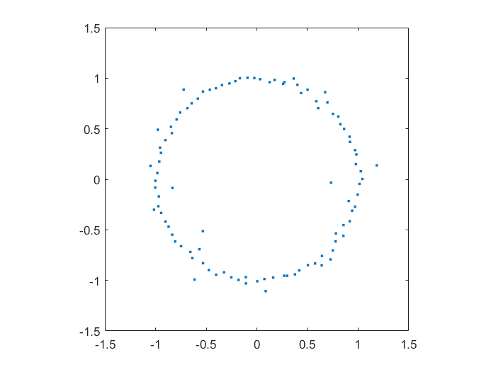
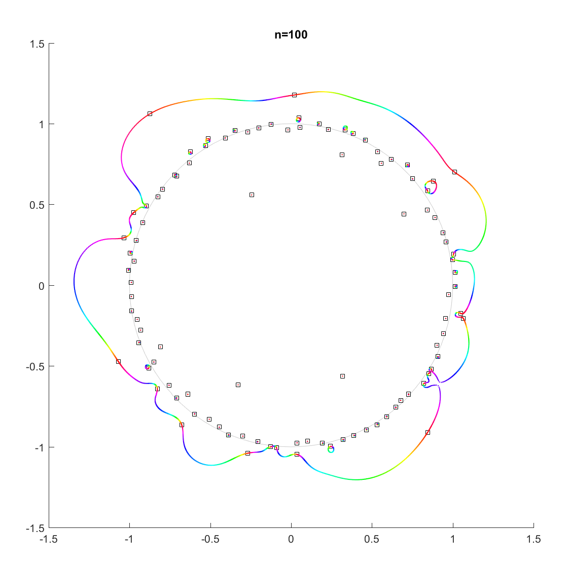
But then I decided to move things around: what if the coefficient on the leading term changed? How would the zeros move? I looked at the polynomial $P_\theta(z)=e^{i\theta} z^n + c_{n-1}z^{n-1}+\ldots+c_1 z + c_0$ where $c_i$ were from some suitable random sequence and $\theta$ could run around $[0,2\pi]$ . Since the leading coefficient would start and end up back at 1, I knew all zeros would return to their starting position. But in between, would they jump around discontinuously or follow orderly paths?

Continuity is actually guaranteed, as shown by (Harris & Martin 1987). As you change the coefficients continuously, the zeros vary continuously too. In fact, for polynomials without multiple zeros, the zeros vary analytically with the coefficients.

As $\theta$ runs from 0 to $2\pi$ the roots move along different orbits. Some end up permuted with each other.

Movement of the zeros of polynomials with random coefficients as the leading coefficient traverses the unit circle. Colour denotes phase, zeros marked by squares.

For low degrees, most zeros participate in a large cycle. Then more and more zeros emerge inside the unit circle and stay mostly fixed as the polynomial changes. As the degree increases they congregate towards the unit circle, while at least one large cycle wraps most of them, often making snaking detours into the zeros near the unit circle and then broad bows outside it.

Movement of the zeros of a random degree 100 polynomial.

In the above example, there is a 21-cycle, as well as a 2-cycle around 2 o’clock. The other zeros stay mostly put.

The real question is what determines the cycles? To understand that, we need to change not just the argument but the magnitude of $c_n$ .

Orbits of roots as the magnitude of the leading coefficient increases from zero to one.

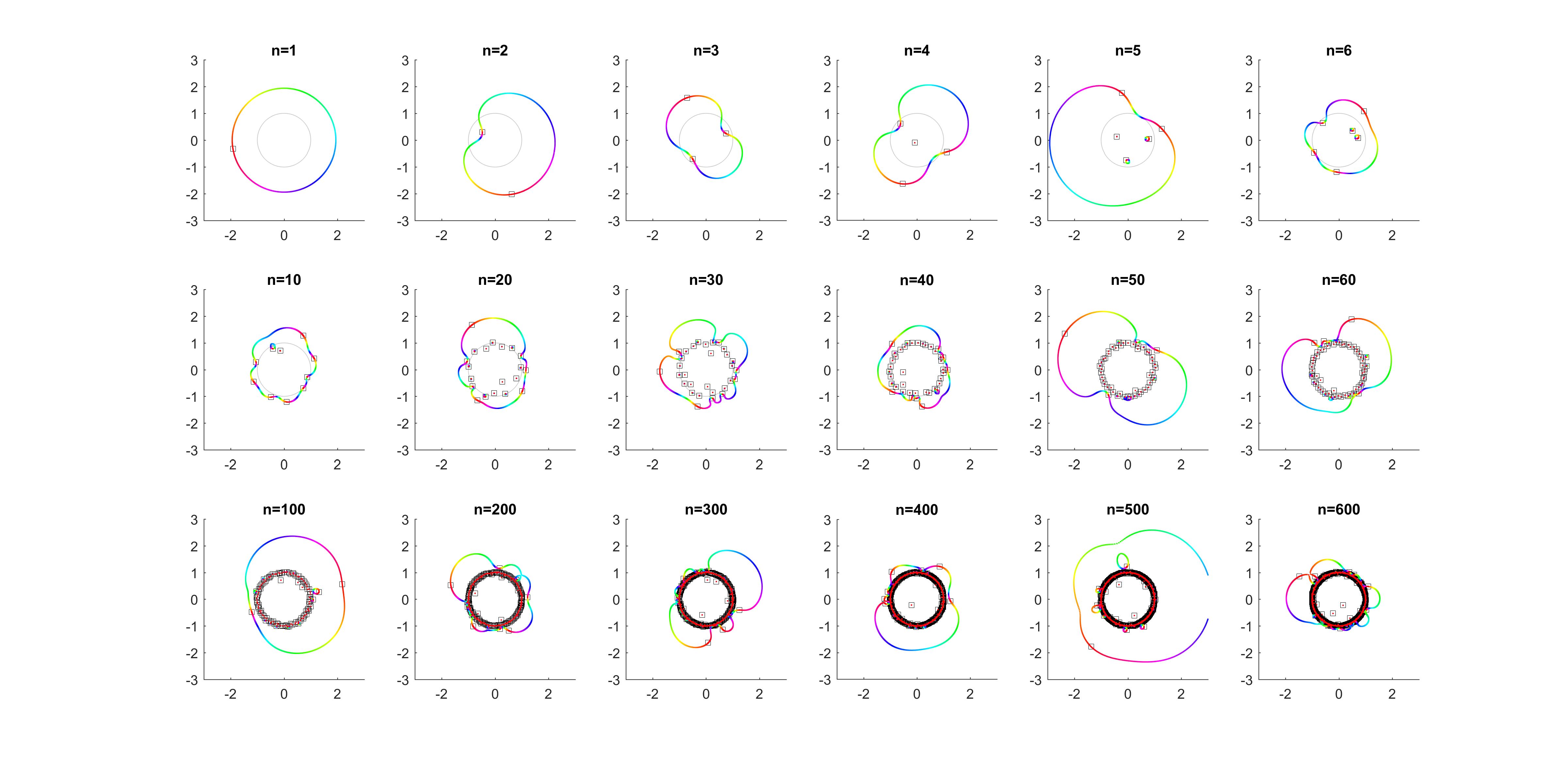
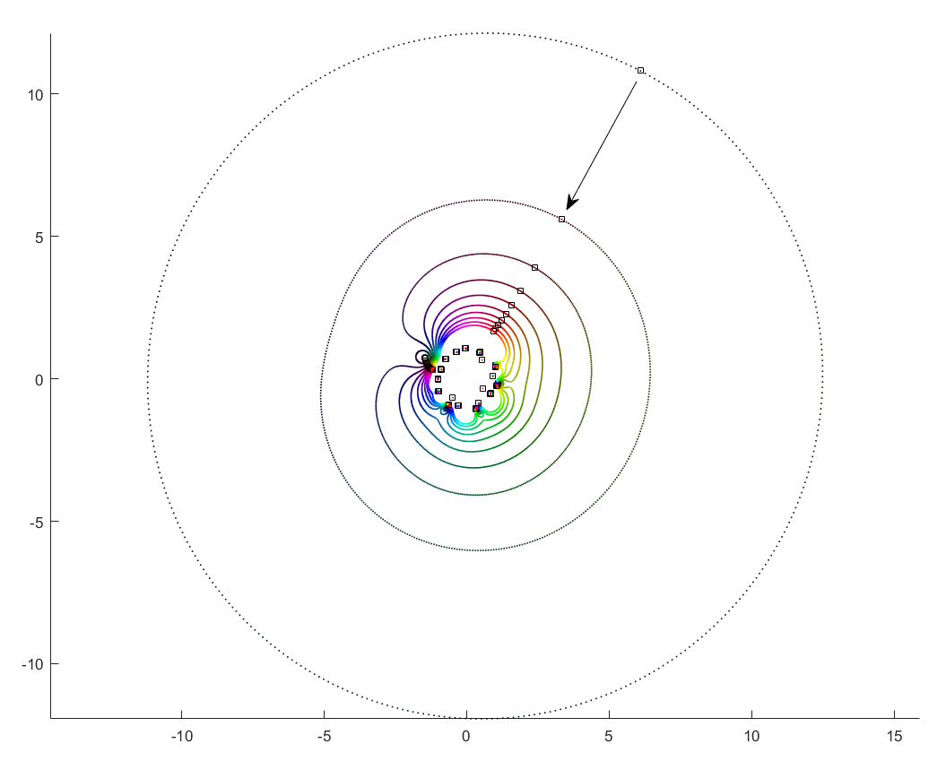
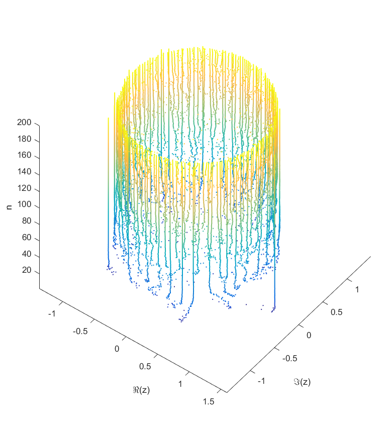
What happens if we slowly increase the magnitude of the leading term, letting $c_n = re^{i\theta}$ for a r that increases from zero? It turns out that a new zero of the function zooms in from infinity towards the unit circle. A way of seeing this is to look at the polynomial as $P_n(z) = c_n z^n + P_{n-1}(z)$ : the second term is nonzero and large in most places, so if $c_n$ is small the $z^n$ factor must be large (and opposite) to outweigh it and cause a zero. The exception is of course close to the zeros of $P_{n-1}(z)$ , where the perturbation just moves them a tiny bit: there is a counterpart for each of the $n-1$ zeros of $P_{n-1}(z)$ among the zeros of $P_{n}(z)$ . While the new root is approaching from outside, if we play with 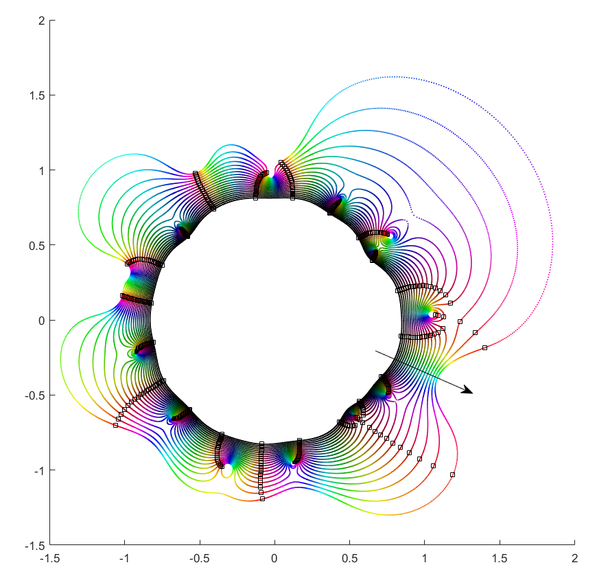$\theta$ it will make a turn around the other zeros: it is alone in its orbit, which also encapsulates all the other zeros. Eventually it will start interacting with them, though.

Orbits of roots as the magnitude of the leading coefficient decreases from 100 to one.

If you instead start out with a large leading term, $|c_n| \gg |c_i|$ , then the polynomial is essentially $P_n(z)=c_nz^n+[\mathrm{small stuff}]$ and the zeros the n-th roots of $-[\mathrm{small stuff}]/c_n$ . All zeros belong to the same roughly circular orbit, moving together as $\theta$ makes a rotation. But as $|c_n|$ decreases the shared orbit develops bulges and dents, and some zeros pinch off from it into their own small circles. When does the pinching off happen? That corresponds to when two zeros coincide during the orbit: one continues on the big orbit, the other one settles down to be local. This is the one case where the analyticity of how they move depending on $c_n$ breaks down. They still move continuously, but there is a sharp turn in their movement direction. Eventually we end up in the small term case, with a single zero on a large radius orbit as $|c_n| \rightarrow 0$ .

This pinching off scenario also suggests why it is rare to find shared orbits in general: they occur if two zeros coincide but with others in between them (e.g. if we number them along the orbit, $z_1=z_k$ , with $z_2$ to $z_{k-1}$ separate). That requires a large pinch in the orbit, but since it is overall pretty convex and circle-like this is unlikely.

Allowing $|c_n|$ to run from $\infty$ to 0 and $\theta$ over $[0,2\pi]$ would cover the entire complex plane (except maybe the origin): for each z, there is some $c_n$ where $c_nz^n+\ldots+c_1z+c_0=0$ . This is fairly obviously $c_n = f(z) = -P_{n-1}(z)/z^n$ . This function has a central pole, surrounded by zeros corresponding to the zeros of $P_{n-1}(z)$ . The orbits we have drawn above correspond to level sets $|f(z)|=\mathrm{const}$ , and the pinching off to saddle points of this surface. To get a multi-zero orbit several zeros need to be close together enough to cause a broad valley.

Graph of the log-magnitude of f(z), the function mapping a point in the plane to the value of c_n that causes a zero to appear there. — Graph of the log-magnitude of f(z), the function mapping a point in the plane to the value of [latex]c_n[/latex] that causes a zero to appear there for [latex]P_n(z)[/latex].

There you have it, a rough theory of dancing zeros.

References

Harris, G., & Martin, C. (1987). Shorter notes: The roots of a polynomial vary continuously as a function of the coefficients. Proceedings of the American Mathematical Society, 390-392.

Hughes, C. P., & Nikeghbali, A. (2008). The zeros of random polynomials cluster uniformly near the unit circle. Compositio Mathematica, 144(03), 734-746.

Desperately Seeking Eternity

Me on BBC3 talking about eternity, the universe, life extension and growing up as a species.

Online text of the essay.

Overall, I am pretty happy with it (hard to get everything I want into a short essay and without using my academic caveats, footnotes and digressions). Except maybe for the title, since “desperate” literally means “without hope”. You do not seek eternity if you do not hope for anything.

Adding cooks to the broth

If there are $k$ key ideas needed to produce some important goal (like AI), there is a constant probability per researcher-year to come up with an idea, and the researcher works for $y$ years, what is the the probability of success? And how does it change if we add more researchers to the team?

The most obvious approach is to think of this as y Bernouilli trials with probability p of success, quickly concluding that the number of successes n at the end of y years will be distributed as $\mathrm{Pr}(n)=\binom{y}{n}p^n(1-p)^{y-n}$ . Unfortunately, then the actual answer to the question will be $\mathrm{Pr}(n\geq k) = \sum_{n=k}^y \binom{y}{n}p^n(1-p)^{y-n}$ which is a real mess…

A somewhat cleaner way of thinking of the problem is to go into continuous time, treating it as a homogeneous Poisson process. There is a rate $\lambda$ of good ideas arriving to a researcher, but they can happen at any time. The time between two ideas will be exponentially distributed with parameter $\lambda$ . So the time $t$ until a researcher has $k$ ideas will be the sum of $k$ exponentials, which is a random variable distributed as the Erlang distribution: $f(t; k,\lambda)=\lambda^k t^{k-1} e^{-\lambda t} / (k-1)!$ .

Just like for the discrete case one can make a crude argument that we are likely to succeed if $y$ is bigger than the mean $k/\lambda$ (or $k/p$ ) we will have a good chance of reaching the goal. Unfortunately the variance scales as $k/\lambda^2$ – if the problems are hard, there is a significant risk of being unlucky for a long time. We have to consider the entire distribution.

Unfortunately the cumulative density function in this case is $\mathrm{Pr}(t<y)=1-\sum_{n=0}^{k-1} e^{-\lambda y} (\lambda y)^n / n!$ which is again not very nice for algebraic manipulation. Still, we can plot it easily.

Before we do that, let us add extra researchers. If there are $N$ researchers, equally good, contributing to the idea generation, what is the new rate of ideas per year? Since we have assumed independence and a Poisson process, it just multiplies the rate by a factor of $N$ . So we replace $\lambda$ with $\lambda N$ everywhere and get the desired answer.

This is a plot of the case $k=10, y=10$ .

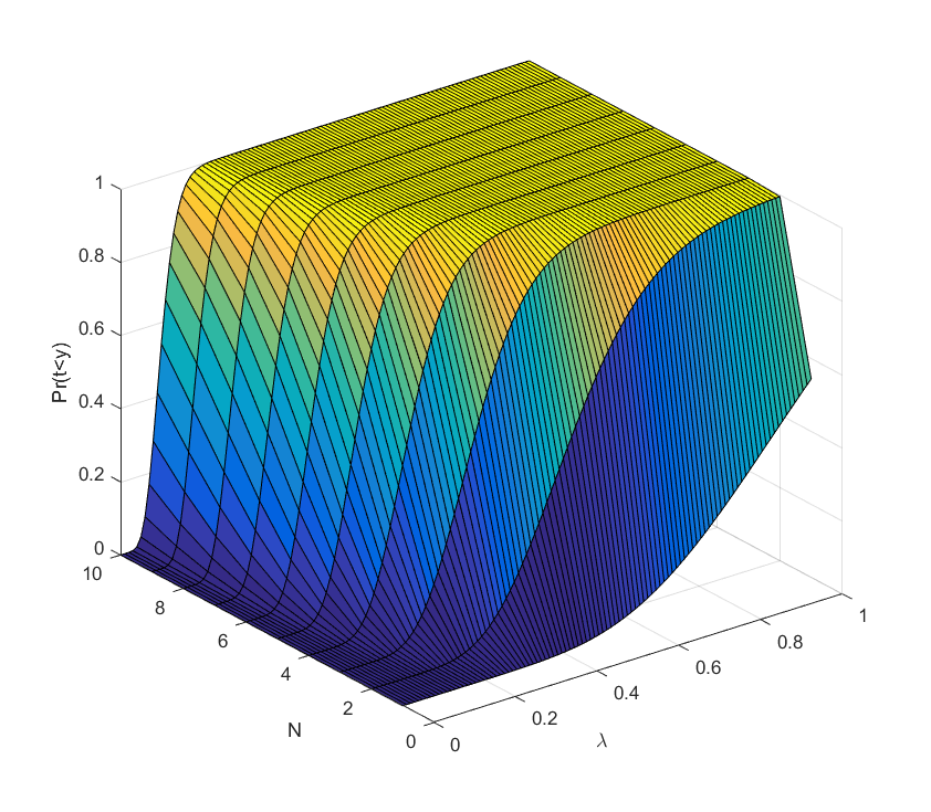
What we see is that for each number of scientists it is a sigmoid curve: if the discovery probability is too low, there is hardly any chance of success, when it becomes comparable to $k/N$ it rises, and sufficiently above we can be almost certain the project will succeed (the yellow plateau). Conversely, adding extra researchers has decreasing marginal returns when approaching the plateau: they make an already almost certain project even more certain. But they do have increasing marginal returns close to the dark blue “floor”: here the chances of success are small, but extra minds increase them a lot.

We can for example plot the ratio of success probability for $\lambda=0.09$ to the one researcher case as we add researchers:

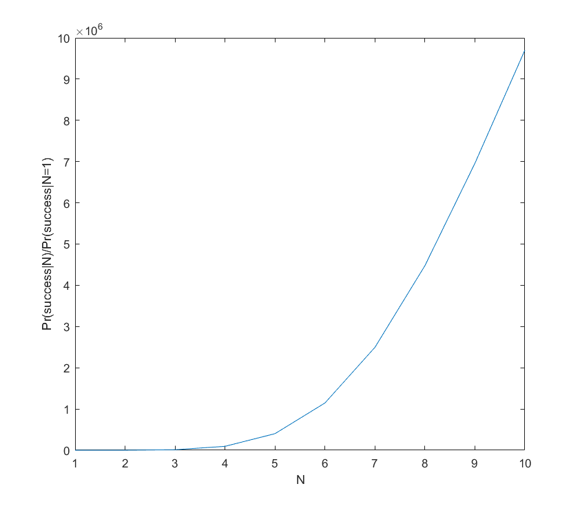
Even with 10 researchers the success probability is just 40%, but clearly the benefit of adding extra researchers is positive. The curve is not quite exponential; it slackens off and will eventually become a big sigmoid. But the overall lesson seems to hold: if the project is a longshot, adding extra brains makes it roughly exponentially more likely to succeed.

It is also worth recognizing that in this model time is on par with discovery rate and number of researchers: what matters is the product $\lambda y N$ and how it compares to $k$ .

This all assumes that ideas arrive independently, and that there are no overheads for having a large team. In reality these things are far more complex. For example, sometimes you need to have idea 1 or 2 before idea 3 becomes possible: that makes the time $t_3$ of that idea distributed as an exponential plus the distribution of $\mathrm{min}(t_1,t_2)$ . If the first two ideas are independent and exponential with rates $\lambda, \mu$ , then the minimum is distributed as an exponential with rate $\lambda+\mu$ . If they instead require each other, we get a non-exponential distribution (the pdf is $\lambda e^{-\lambda t} + \mu e^{-\mu t} - (\lambda+\mu)e^{-(\lambda+\mu)t}$ ). Some discoveries or bureaucratic scalings may change the rates. One can construct complex trees of intellectual pathways, unfortunately quickly making the distributions impossible to write out (but still easy to run Monte Carlo on). However, as long as the probabilities and the induced correlations small, I think we can linearise and keep the overall guess that extra minds are exponentially better.

In short: if the cooks are unlikely to succeed at making the broth, adding more is a good idea. If they already have a good chance, consider managing them better.

Julia lace gaskets

While surfing the web I came across a neat Julia set, defined by iterating $z_{n+1}=f(z_n)=z_n^2+c/z_n^3$ for some complex constant c. Here are some typical pictures, and two animations: one moving around a circle in the c-plane, one moving slowly down from c=1 to c=0.

The points behind the set

What is going on?

The first step in analysing fractals like this is to find the fixed points and their preimages. $z=\infty$ is clearly mapped to itself. The $z^2$ term will tend to make large magnitude iterates approach infinity, so it is an attractive fixed point.

$z=0$ is a preimage of infinity: iterates falling on zero will be mapped onto infinity. Nearby points will also end up attracted to infinity, so we have a basin of attraction to infinity around the origin. Preimages of the origin will be mapped to infinity in two steps: $0=z^2+c/z^3$ has the solutions $z=(-c)^{1/5}$ – this is where the pentagonal symmetry comes from, since these five points are symmetric. Their preimages and so on will also be mapped to infinity, so we have a hierarchy of basins of attraction sending points away forming some gasket-like structure. The Julia set consists of the points that never gets mapped away, the boundary of this hierarchy of basins.

The other fixed points are defined by $z=z^2+c/z^3$ , which can be rearranged into $z^5-z^4+c=0$ . They don’t have any neat expression and actually do not affect the big picture dynamics as much. The main reason seems to be that they are unstable. However, their location and the derivative close to them affect the shapes in the Julia set as we will see. Their preimages will be surrounded by the same structures (scaled and rotated) as they have.

Below are examples with preimages of zero marked as white circles, fixed points as red crosses, and critical points as black squares.

The set behind the points

A simple way of mapping the dynamics is to look at the (generalized) Mandelbrot set for the function, taking a suitable starting point $z_0=(3c/2)^{1/5}$ and mapping out its fate in the c-plane. Why that particular point? Because it is one of the critical point where $f'(z)=0$ , and a theorem by Julia and Fatou tells us that its fate indicates whether the Julia set is filled or dust-like: bounded orbits of the critical points of a map imply a connected Julia set. When c is in the Mandelbrot set the Julia image has “thick” regions with finite area that do not escape to infinity. When c is outside, then most points end up at infinity, and what remains is either dust or a thin gasket with no area.

The set is much smaller than the vanilla $f(z)=z^2+c$ Mandelbrot, with a cuspy main body surrounded by a net reminiscent of the gaskets in the Julia set. It also has satellite vanilla Mandelbrots, which is not surprising at all: the square term tends to dominate in many locations. As one zooms into the region near the origin a long spar covered in Mandelbrot sets runs towards the origin, surrounded by lacework.

One surprising thing is that the spar does not reach the origin – it stops at $c=4.5 \cdot 10^{-5}$ . Looking at the dynamics, above this point the iterates of the critical point jump around in the interval [0,1], forming a typical Feigenbaum cascade of period doubling as you go out along the spar (just like on the spar of the vanilla Mandelbrot set). But at this location points now are mapped outside the interval, running off to infinity: one of the critical points breaches a basin boundary, causing iterates to run off and the earlier separate basins to merge. Below this point the dynamics is almost completely dominated by the squaring, turning the Julia set into a product of a Cantor set and a circle (a bit wobbly for higher c; it is all very similar to KAM torii). The empty spaces correspond to the regions where preimages of zero throw points to infinity, while along the wobbly circles points get their argument angles multiplied by two for every iteration by the dominant quadratic term: they are basically shift maps. For c=0 it is just the filled unit disk.

So when we allow c to move around a circle as in the animations, the part that passes through the Mandelbrot set has thick regions that thin as we approach the edge of the set. Since the edge is highly convoluted the passage can be quite complex (especially if the circle is “tangent” to it) and the regions undergo complex twisting and implosions/explosions. During the rest of the orbit the preimages just quietly rotate, forming a fractal gasket. A gasket that sometimes looks like a model of the hyperbolic plane, since each preimage has five other preimages, naturally forming an exponential hierarchy that has to be squeezed into a finite roughly circular space.

The Annihilation Score as Satirical Sociology

Today I read The Annihilation Score by Charles Stross during a flight. It is the sixth Laundry novel, and in many ways the weakest. But it might be the intellectually and satirically best.

The Laundry novels are a mix of horror, spy story, geekiness, and satire. This is both a reader-winning combination (transitions from one side of the mixture to another can provide intense contrast, and Stross can give readers a bit of everything) and a balancing problem: each story needs to maintain the right mixture, and the readers often have their own favourite ratios. The Annihilation Score goes further in the direction of satire, reducing the horror and geekiness fairly significantly. This no doubt makes many Laundry fans unhappy. Me too, to some extent: there is nothing more delightful than noticing wordplay based on obscure hermetica and computer science, or the distinctly unsettling implications of thinking through some of the metaphysical assumptions of the setting. However, I think Stross hit on something different in this novel: an important argument disguised as satire.

On the surface the novel suffers from bad pacing: the bulk of it is about management. Not intense action, but rather the issue of how to set up an office, from personnel management to furniture to keeping the funding body happy despite contradictory goals. There is plenty of agency-spotting, with numerous acronymical organisations criss-crossing the story with their interleaved agendas. And finally, in the last fifth, a climactic battle. Typically Laundry novels spend a lot of times establishing a mood and tension for a relatively brief finale where they get unleashed. The Annihilation Score takes this even further, but at least I did not feel much of a build-up. In fact, despite the pressure on the main character she comes across as almost a Westminster Mary Sue: she persists and succeeds at nearly everything, from turning what ought to be a social nightmare into a cozy core team, to handling unseen budgetary constraints.

However, on a deeper level this is not a horror story about inhuman entities from other dimensions threatening to invade our world and their misguided human servants. This is a horror story about the inhuman entity inhabiting Whitehall: government.

Taking jabs at the absurdity, stupidity and inhumanity of bureaucracy has been a staple in the Laundry books. What makes the Annihilation Score stand out is that it actually has a fairly well thought out argument and exposition of why. The basics are familiar from the earlier novels: the iron law of bureaucracy (framed here as the emergent instrumental goal of organisations to preserve themselves), Parkinson’s law, the Snafu principle, empire building, not invented here, in-group out-group dynamics, Something Must Be Done, and so on. The novel does a sociological dive into the internal culture of the subset of bureaucracy dealing with policing. Here there exists a strong ethos about what purpose it actually has, which both serves to recruit and advance people with a compatible mindset and actually maintain some mission focus. Presumably because it would be very noticeable if the police force began too drift too far from its necessary function; compare this with how some branches of academia are kept honest by constant interaction with an unyielding real world, and others diffuse into obscure absurdity since there are only social forces constraining them. But even when a purpose has an apparently clear meaning it can get subtly (or not so subtly) twisted. This is especially true at the top, where the constraints of external practical reality are weakest.

Stross examines the case where bureaucracy recognizes it has an out-of-context problem. Something important yet unknown is intruding, and clearly something must be done to handle it. The problem is of course that following the politician’s syllogism means that whatever fast and decisive action is taken is not going to be based on good knowledge. Worse, if the organisation is centred on dealing with something Very Important like national security it will hence be (1) extremely motivated to do it, (2) discount signals from unimportant (as described by its own value system) organisations or sources. A not so subtle analogy to the Annihilation Score is government handling of many emerging technologies such as encryption. Internal expertise is lacking not just on the technology itself and its full implications, but there is also a lack of expertise in judging the consequences of different actions and expertise in recognizing this kind of expertise.

This is where I think the novel actually succeeds: it plays out a satirical scenario, but the parts are all-too-familiar. Well-meaning people work hard to ensure something agreed to be good, and the result is Moloch. The Sleeper in the Pyramid is not half as scary as the Dweller in Whitehall. Because the later is real.

Andart II

Part of Anders' Exoself

Author: admin