Robin Hanson mentions that some people take him to task for working on one scenario (WBE) that might not be the most likely future scenario (“standard AI”); he responds by noting that there are perhaps 100 times more people working on standard AI than WBE scenarios, yet the probability of AI is likely not a hundred times higher than WBE. He also notes that there is a tendency for thinkers to clump onto a few popular scenarios or issues. However:
In addition, due to diminishing returns, intellectual attention to future scenarios should probably be spread out more evenly than are probabilities. The first efforts to study each scenario can pick the low hanging fruit to make faster progress. In contrast, after many have worked on a scenario for a while there is less value to be gained from the next marginal effort on that scenario.
This is very similar to my own thinking about research effort. Should we focus on things that are likely to pan out, or explore a lot of possibilities just in case one of the less obvious cases happens? Given that early progress is quick and easy, we can often get a noticeable fraction of whatever utility the topic has by just a quick dip. The effective altruist heuristic of looking at neglected fields also is based on this intuition.
A model
But under what conditions does this actually work? Here is a simple model:
There are possible scenarios, one of which () will come about. They have probability . We allocate a unit budget of effort to the scenarios: . For the scenario that comes about, we get utility (diminishing returns).
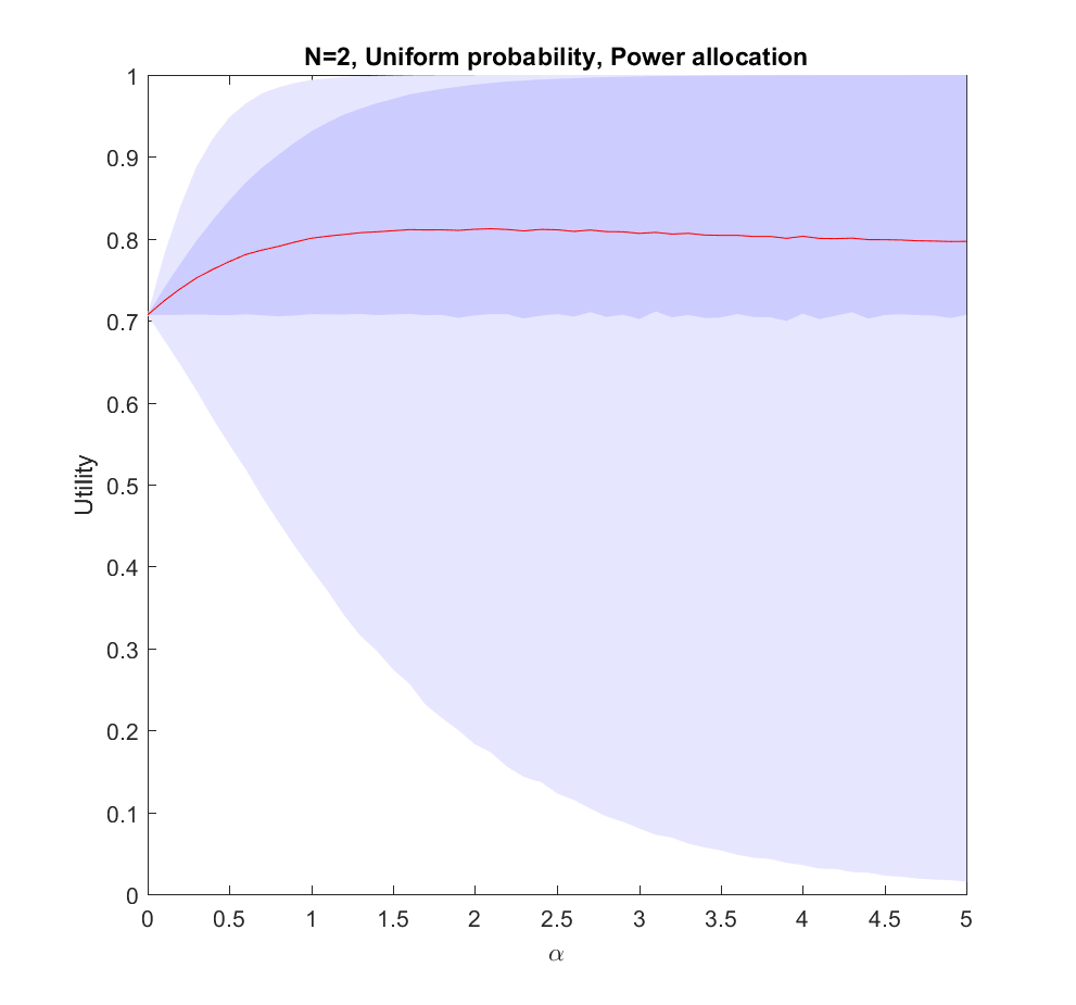
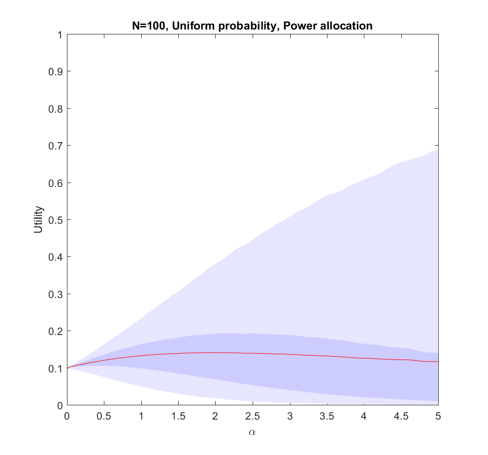
Here is what happens if we allocate proportional to a power of the scenarios, . corresponds to even allocation, 1 proportional to the likelihood, >1 to favoring the most likely scenarios. In the following I will run Monte Carlo simulations where the probabilities are randomly generated each instantiation. The outer bluish envelope represents the 95% of the outcomes, the inner ranges from the lower to the upper quartile of the utility gained, and the red line is the expected utility.
Utility of allocating effort as a power of the probability of scenarios. Red line is expected utility, deeper blue envelope is lower and upper quartiles, lighter blue 95% interval.
This is the case: we have two possible scenarios with probability and (where is uniformly distributed in [0,1]). Just allocating evenly gives us utility on average, but if we put in more effort on the more likely case we will get up to 0.8 utility. As we focus more and more on the likely case there is a corresponding increase in variance, since we may guess wrong and lose out. But 75% of the time we will do better than if we just allocated evenly. Still, allocating nearly everything to the most likely case means that one does lose out on a bit of hedging, so the expected utility declines slowly for large .
Utility of allocating effort as a power of the probability of scenarios. Red line is expected utility, deeper blue envelope is lower and upper quartiles, lighter blue 95% interval. 100 possible scenarios, with uniform probability on the simplex.
The case (where the probabilities are allocated based on a flat Dirichlet distribution) behaves similarly, but the expected utility is smaller since it is less likely that we will hit the right scenario.
What is going on?
This doesn’t seem to fit Robin’s or my intuitions at all! The best we can say about uniform allocation is that it doesn’t produce much regret: whatever happens, we will have made some allocation to the possibility. For large N this actually works out better than the directed allocation for a sizable fraction of realizations, but on average we get less utility than betting on the likely choices.
The problem with the model is of course that we actually know the probabilities before making the allocation. In reality, we do not know the likelihood of AI, WBE or alien invasions. We have some information, and we do have priors (like Robin’s view that ), but we are not able to allocate perfectly. A more plausible model would give us probability estimates instead of the actual probabilities.
We know nothing
Let us start by looking at the worst possible case: we do not know what the true probabilities are at all. We can draw estimates from the same distribution – it is just that they are uncorrelated with the true situation, so they are just noise.
Utility of allocating effort as a power of the probability of scenarios, but the probabilities are just random guesses. Red line is expected utility, deeper blue envelope is lower and upper quartiles, lighter blue 95% interval. 100 possible scenarios, with uniform probability on the simplex.
In this case uniform distribution of effort is optimal. Not only does it avoid regret, it has a higher expected utility than trying to focus on a few scenarios (). The larger N is, the less likely it is that we focus on the right scenario since we know nothing. The rationality of ignoring irrelevant information is pretty obvious.
Note that if we have to allocate a minimum effort to each investigated scenario we will be forced to effectively increase our above 0. The above result gives the somewhat optimistic conclusion that the loss of utility compared to an even spread is rather mild: in the uniform case we have a pretty low amount of effort allocated to the winning scenario, so the low chance of being right in the nonuniform case is being balanced by having a slightly higher effort allocation on the selected scenarios. For high there is a tail of rare big “wins” when we hit the right scenario that drags the expected utility upwards, even though in most realizations we bet on the wrong case. This is very much the hedgehog predictor story: ocasionally they have analysed the scenario that comes about in great detail and get intensely lauded, despite looking at the wrong things most of the time.
We know a bit
We can imagine that knowing more should allow us to gradually interpolate between the different results: the more you know, the more you should focus on the likely scenarios.
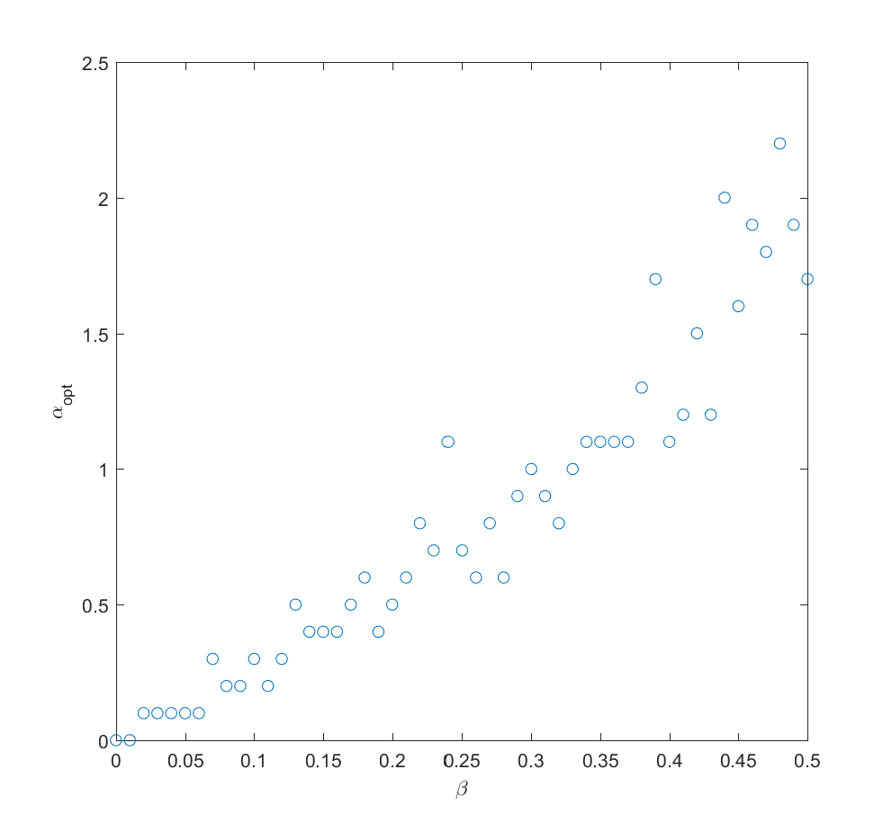
Optimal alpha as a function of how much information we have about the true probabilities (noise due to Monte Carlo and discrete steps of alpha). N=2 (N=100 looks similar).
If we take the mean of the true probabilities with some randomly drawn probabilities (the “half random” case) the curve looks quite similar to the case where we actually know the probabilities: we get a maximum for . In fact, we can mix in just a bit () of the true probability and get a fairly good guess where to allocate effort (i.e. we allocate effort as where is uncorrelated noise probabilities). The optimal alpha grows roughly linearly with , in this case.
We learn
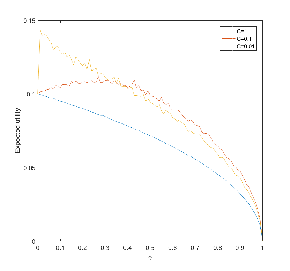
Adding a bit of realism, we can consider a learning process: after allocating some effort to the different scenarios we get better information about the probabilities, and can now reallocate. A simple model may be that the standard deviation of noise behaves as where is the effort placed in exploring the probability of scenario . So if we begin by allocating uniformly we will have noise at reallocation of the order of . We can set , where is some constant denoting how tough it is to get information. Putting this together with the above result we get . After this exploration, now we use the remaining effort to work on the actual scenarios.
Expected utility as a function of amount of probability-estimating effort (gamma) for C=1 (hard to update probabilities), C=0.1 and C=0.01 (easy to update). N=100.
This is surprisingly inefficient. The reason is that the expected utility declines as and the gain is just the utility difference between the uniform case and optimal , which we know is pretty small. If C is small (i.e. a small amount of effort is enough to figure out the scenario probabilities) there is an optimal nonzero . This optimum decreases as C becomes smaller. If C is large, then the best approach is just to spread efforts evenly.
Conclusions
So, how should we focus? These results suggest that the key issue is knowing how little we know compared to what can be known, and how much effort it would take to know significantly more.
If there is little more that can be discovered about what scenarios are likely, because our state of knowledge is pretty good, the world is very random, or improving knowledge about what will happen will be costly, then we should roll with it and distribute effort either among likely scenarios (when we know them) or spread efforts widely (when we are in ignorance).
If we can acquire significant information about the probabilities of scenarios, then we should do it – but not overdo it. If it is very easy to get information we need to just expend some modest effort and then use the rest to flesh out our scenarios. If it is doable but costly, then we may spend a fair bit of our budget on it. But if it is hard, it is better to go directly on the object level scenario analysis as above. We should not expect the improvement to be enormous.
Here I have used a square root diminishing return model. That drives some of the flatness of the optima: had I used a logarithm function things would have been even flatter, while if the returns diminish more mildly the gains of optimal effort allocation would have been more noticeable. Clearly, understanding the diminishing returns, number of alternatives, and cost of learning probabilities better matters for setting your strategy.
In the case of future studies we know the number of scenarios are very large. We know that the returns to forecasting efforts are strongly diminishing for most kinds of forecasts. We know that extra efforts in reducing uncertainty about scenario probabilities in e.g. climate models also have strongly diminishing returns. Together this suggests that Robin is right, and it is rational to stop clustering too hard on favorite scenarios. Insofar we learn something useful from considering scenarios we should explore as many as feasible.
By Anders Sandberg, Future of Humanity Institute, Oxford Martin School, University of Oxford
Thinking of the future is often done as entertainment. A surprising number of serious-sounding predictions, claims and prophecies are made with apparently little interest in taking them seriously, as evidenced by how little they actually change behaviour or how rarely originators are held responsible for bad predictions. Rather, they are stories about our present moods and interests projected onto the screen of the future. Yet the future matters immensely: it is where we are going to spend the rest of our lives. As well as where all future generations will live – unless something goes badly wrong.
Olle Häggström’s book is very much a plea for taking the future seriously, and especially for taking exploring the future seriously. As he notes, there are good reasons to believe that many technologies under development will have enormous positive effects… and also good reasons to suspect that some of them will be tremendously risky. It makes sense to think about how we ought to go about avoiding the risks while still reaching the promise.
Current research policy is often directed mostly towards high quality research rather than research likely to make a great difference in the long run. Short term impact may be rewarded, but often naively: when UK research funding agencies introduced impact evaluation a few years back, their representatives visiting Oxford did not respond to the question on whether impact had to be positive. Yet, as Häggström argues, obviously the positive or negative impact of research must matter! A high quality investigation into improved doomsday weapons should not be pursued. Investigating the positive or negative implications of future research and technology has high value, even if it is difficult and uncertain.
Inspired by James Martin’s The Meaning of the 21st Century this book is an attempt to make a broad map sketch of parts of the future that matters, especially the uncertain corners where we have reason to think dangerous dragons lurk. It aims more at scope than the detail of many of the covered topics, making it an excellent introduction and pointer towards the primary research.
One obvious area is climate change, not just in terms of its direct (and widely recognized risks) but the new challenges posed by geoengineering. Geoengineering may both be tempting to some nations and possible to perform unilaterally, yet there are a host of ethical, political, environmental and technical risks linked to it. It also touches on how far outside the box we should search for solutions: to many geoengineering is already too far, but other proposals such as human engineering (making us more eco-friendly) go much further. When dealing with important challenges, how do we allocate our intellectual resources?
Other areas Häggström reviews include human enhancement, artificial intelligence, and nanotechnology. In each of these areas tremendously promising possibilities – that would merit a strong research push towards them – are intermixed with different kinds of serious risks. But the real challenge may be that we do not yet have the epistemic tools to analyse these risks well. Many debates in these areas contain otherwise very intelligent and knowledgeable people making overconfident and demonstrably erroneous claims. One can also argue that it is not possible to scientifically investigate future technology. Häggström disagrees with this: one can analyse it based on currently known facts and using careful probabilistic reasoning to handle the uncertainty. That results are uncertain does not mean they are useless for making decisions.
He demonstrates this by analysing existential risks, scenarios for the long term future humanity and what the “Fermi paradox” may tell us about our chances. There is an interesting interplay between uncertainty and existential risk. Since our species can end only once, traditional frequentist approaches run into trouble Bayesian methods do not. Yet reasoning about events that are unprecedented also makes our arguments terribly sensitive to prior assumptions, and many forms of argument are more fragile than they first look. Intellectual humility is necessary for thinking about audacious things.
In the end, this book is as much a map of relevant areas of philosophy and mathematics containing tools for exploring the future, as it is a direct map of future technologies. One can read it purely as an attempt to sketch where there may be dragons in the future landscape, but also as an attempt at explaining how to go about sketching the landscape. If more people were to attempt that, I am confident that we would fence in the dragons better and direct our policies towards more dragon-free regions. That is a possibility worth taking very seriously.
[Conflict of interest: several of my papers are discussed in the book, both critically and positively.]
Yesterday I gave a talk at the joint Bloomberg-London Futurist meeting “The state of the future” about the future of decisionmaking. Parts were updates on my policymaking 2.0 talk (turned into this chapter), but I added a bit more about individual decisionmaking, rationality and forecasting.
The big idea of the talk: ensemble methods really work in a lot of cases. Not always, not perfectly, but they should be among the first tools to consider when trying to make a robust forecast or decision. They are Bayes’ broadsword:
OK, so in forecasting it looks like using multiple methods, theories and data sources (including experts) is a way to get better results.
Statistical machine learning
A standard problem in machine learning is to classify something into the right category from data, given a set of training examples. For example, given medical data such as age, sex, and blood test results, diagnose what a particular disease a patient might suffer from. The key problem is that it is non-trivial to construct a classifier that works well on data different from the training data. It can work badly on new data, even if it works perfectly on the training examples. Two classifiers that perform equally well during training may perform very differently in real life, or even for different data.
The obvious solution is to combine several classifiers and average (or vote about) their decisions: ensemble based systems. This reduces the risk of making a poor choice, and can in fact improve overall performance if they can specialize for different parts of the data. This also has other advantages: very large datasets can be split into manageable chunks that are used to train different components of the ensemble, tiny datasets can be “stretched” by random resampling to make an ensemble trained on subsets, outliers can be managed by “specialists”, in data fusion different types of data can be combined, and so on. Multiple weak classifiers can be combined into a strong classifier this way.
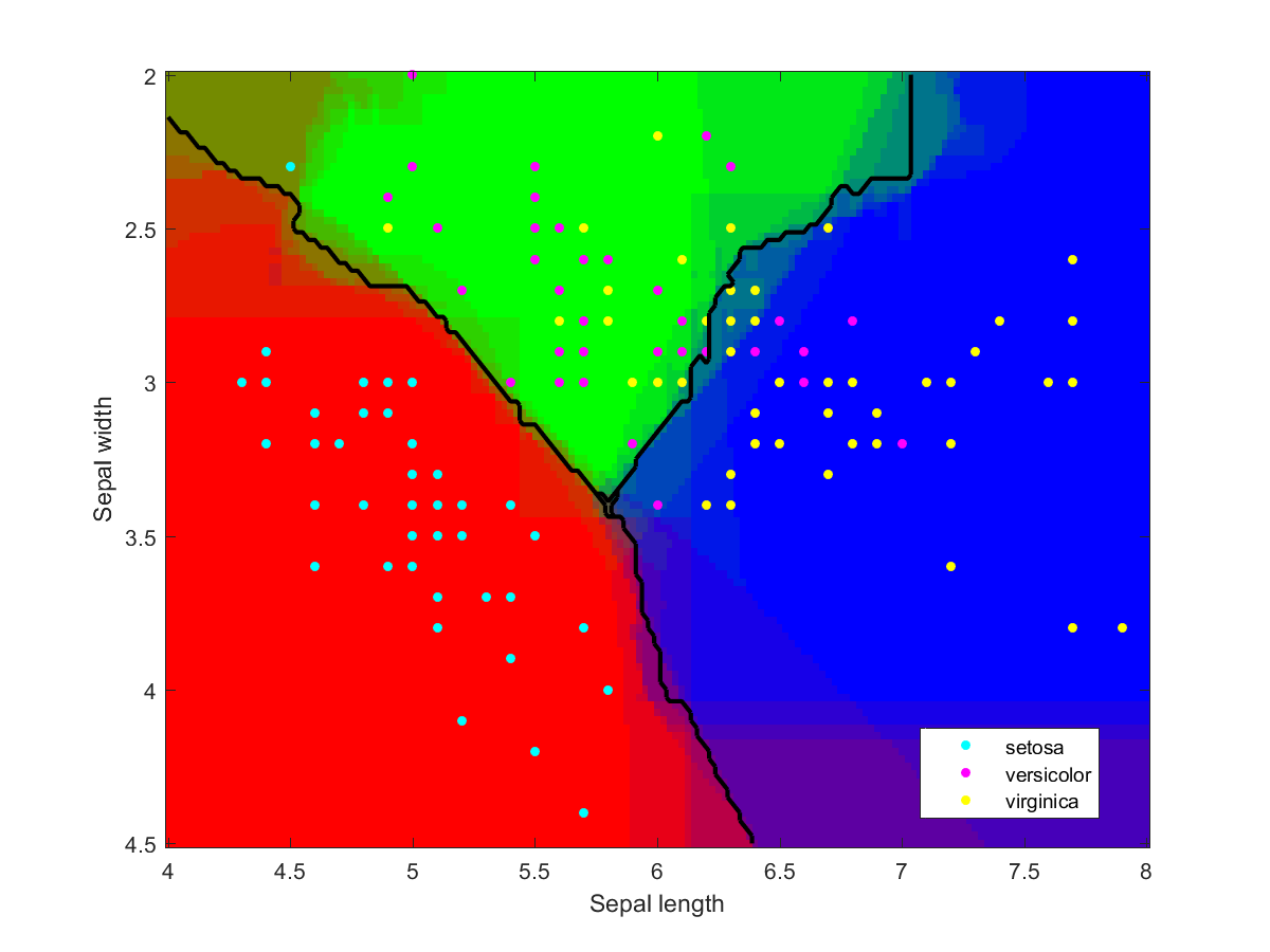
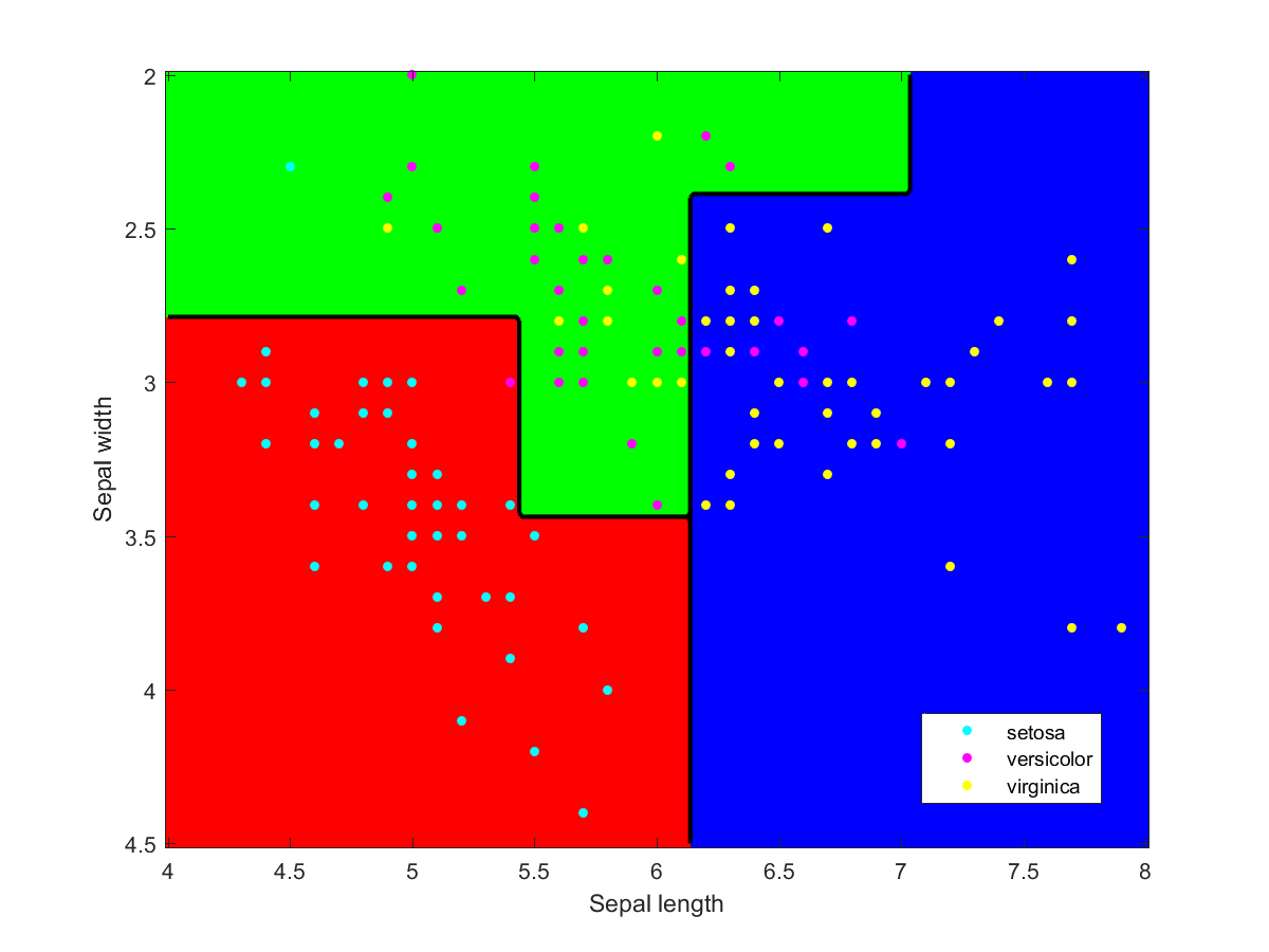
Iris data classified using an ensemble of classification methods (LDA, NBC, various kernels, decision tree). Note how the combination of classifiers also roughly indicates the overall reliability of classifications in a region.
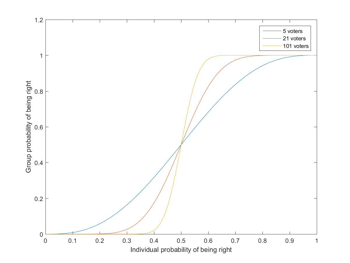
Condorcet’s jury theorem is perhaps the classic result in group problem solving: if a group of people hold a majority vote, and each has a probability p>1/2 of voting for the correct choice, then the probability the group will vote correctly is higher than p and will tend to approach 1 as the size of the group increases. This presupposes that votes are independent, although stronger forms of the theorem have been proven. (In reality people may have different preferences so there is no clear “right answer”)
Probability that groups of different sizes will reach the correct decision as a function of the individual probability of voting right.
By now the pattern is likely pretty obvious. Weak decision-makers (the voters) are combined through a simple procedure (the vote) into better decision-makers.
Group problem solving is known to be pretty good at smoothing out individual biases and errors. In The Wisdom of Crowds Surowiecki suggests that the ideal crowd for answering a question in a distributed fashion has diversity of opinion, independence (each member has an opinion not determined by the other’s), decentralization (members can draw conclusions based on local knowledge), and the existence of a good aggregation process turning private judgements into a collective decision or answer.
Perhaps the grandest example of group problem solving is the scientific process, where peer review, replication, cumulative arguments, and other tools make error-prone and biased scientists produce a body of findings that over time robustly (if sometimes slowly) tends towards truth. This is anything but independent: sometimes a clever structure can improve performance. However, it can also induce all sorts of nontrivial pathologies – just consider the detrimental effects status games have on accuracy or focus on the important topics in science.
Small group problem solving on the other hand is known to be great for verifiable solutions (everybody can see that a proposal solves the problem), but unfortunately suffers when dealing with “wicked problems” lacking good problem or solution formulation. Groups also have scaling issues: a team of N people need to transmit information between all N(N-1)/2 pairs, which quickly becomes cumbersome.
One way of fixing these problems is using software and formal methods.
The Good Judgement Project (partially run by Tetlock and with Armstrong on the board of advisers) participated in the IARPA ACE program to try to improve intelligence forecasts. They used volunteers and checked their forecast accuracy (not just if they got things right, but if claims that something was 75% likely actually came true 75% of the time). This led to a plethora of fascinating results. First, accuracy scores based on the first 25 questions in the tournament predicted subsequent accuracy well: some people were consistently better than others, and it tended to remain constant. Training (such a debiasing techniques) and forming teams also improved performance. Most impressively, using the top 2% “superforecasters” in teams really outperformed the other variants. The superforecasters were a diverse group, smart but by no means geniuses, updating their beliefs frequently but in small steps.
The key to this success was that a computer- and statistics-aided process found the good forecasters and harnessed them properly (plus, the forecasts were on a shorter time horizon than the policy ones Tetlock analysed in his previous book: this both enables better forecasting, plus the all-important feedback on whether they worked).
Another good example is the Galaxy Zoo, an early crowd-sourcing project in galaxy classification (which in turn led to the Zooniverse citizen science project). It is not just that participants can act as weak classifiers and combined through a majority vote to become reliable classifiers of galaxy type. Since the type of some galaxies is agreed on by domain experts they can used to test the reliability of participants, producing better weightings. But it is possible to go further, and classify the biases of participants to create combinations that maximize the benefit, for example by using overly “trigger happy” participants to find possible rare things of interest, and then check them using both conservative and neutral participants to become certain. Even better, this can be done dynamically as people slowly gain skill or change preferences.
The right kind of software and on-line “institutions” can shape people’s behavior so that they form more effective joint cognition than they ever could individually.
Conclusions
The big idea here is that it does not matter that individual experts, forecasting methods, classifiers or team members are fallible or biased, if their contributions can be combined in such a way that the overall output is robust and less biased. Ensemble methods are examples of this.
While just voting or weighing everybody equally is a decent start, performance can be significantly improved by linking it to how well the participants perform. Humans can easily be motivated by scoring (but look out for disalignment of incentives: the score must accurately reflect real performance and must not be gameable).
Having a flexible structure that can change is a good approach to handling a changing world. If people have disincentives to change their mind or change teams, they will not update beliefs accurately.
I got a good question after the talk: if we are supposed to keep our models simple, how can we use these complicated ensembles? The answer is of course that there is a difference between using a complex and a complicated approach. The methods that tend to be fragile are the ones with too many free parameters, too much theoretical burden: they are the complex “hedgehogs”. But stringing together a lot of methods and weighting them appropriately merely produces a complicated model, a “fox”. Component hedgehogs are fine as long as they are weighed according to how well they actually perform.
(In fact, adding together many complex things can make the whole simpler. My favourite example is the fact that the Kolmogorov complexity of integers grows boundlessly on average, yet the complexity of the set of all integers is small – and actually smaller than some integers we can easily name. The whole can be simpler than its parts.)
In the end, we are trading Occam’s razor for a more robust tool: Bayes’ Broadsword. It might require far more strength (computing power/human interaction) to wield, but it has longer reach. And it hits hard.
Appendix: individual classifiers
I used Matlab to make the illustration of the ensemble classification. Here are some of the component classifiers. They are all based on the examples in the Matlab documentation. My ensemble classifier is merely a maximum vote between the component classifiers that assign a class to each point.
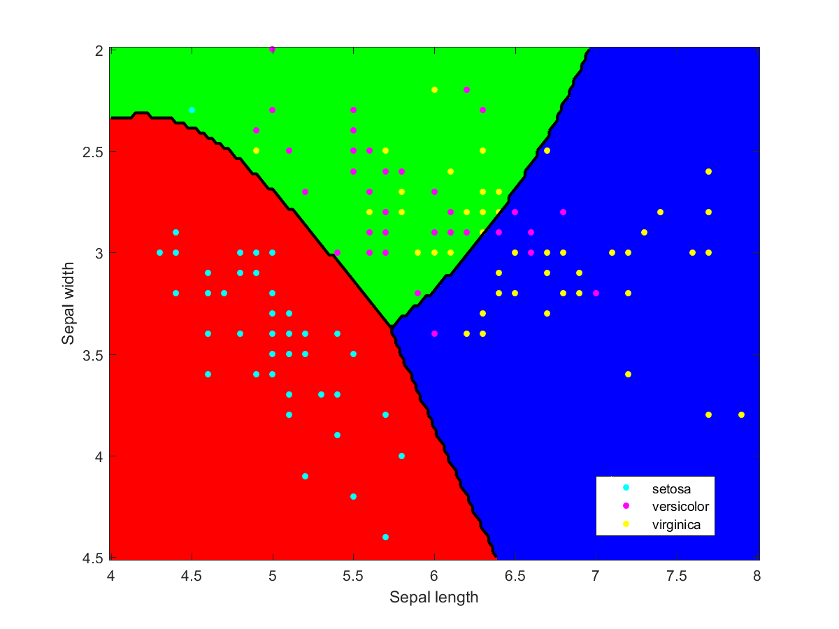
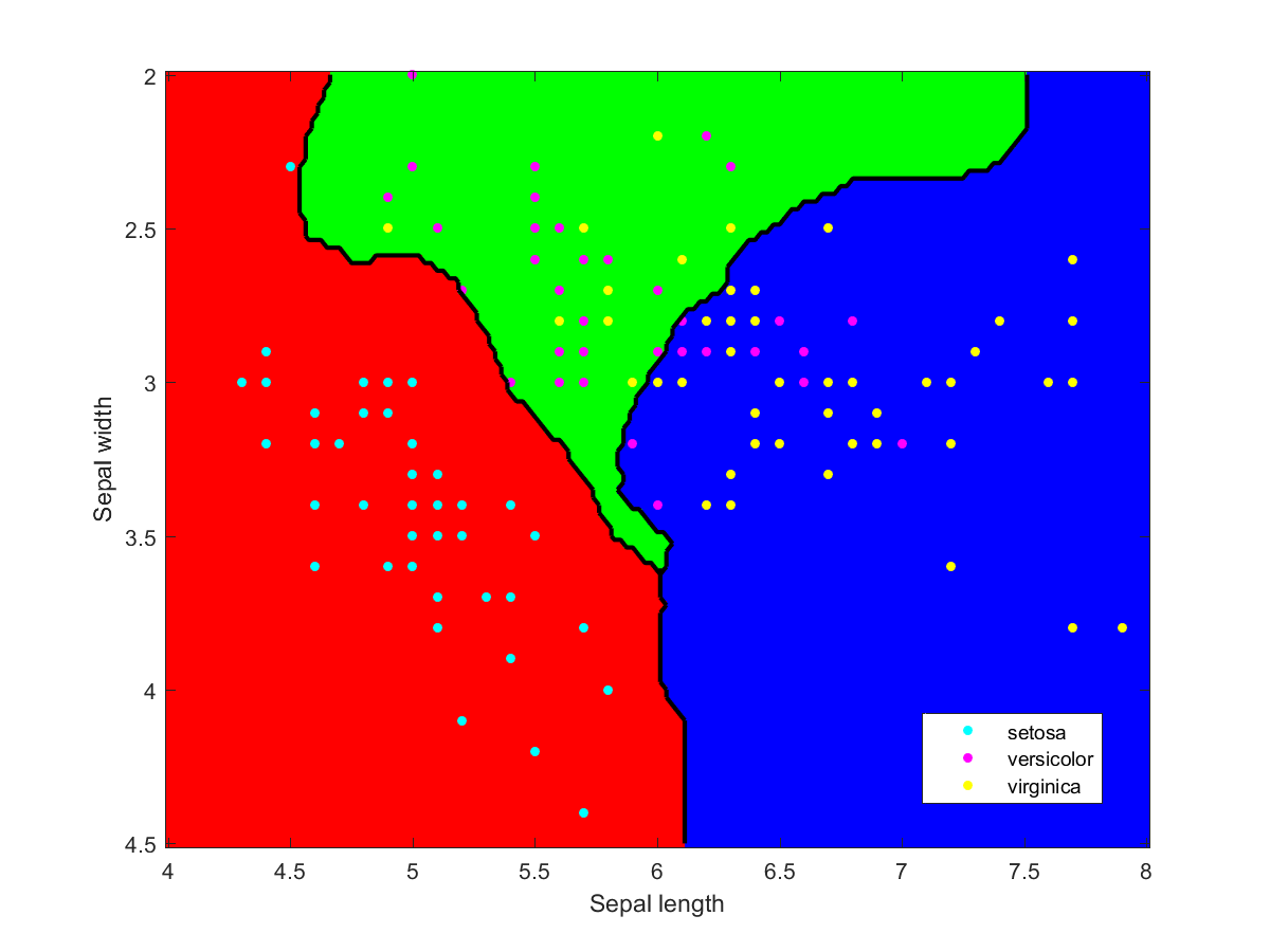
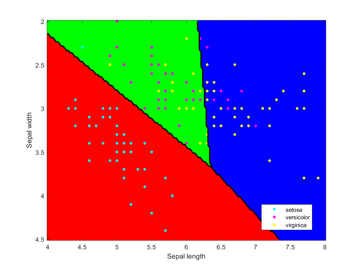
Iris data classified using a naive Bayesian classifier assuming Gaussian distributions.Iris data classified using a decision tree.Iris data classified using Gaussian kernels.Iris data classified using linear discriminant analysis.


Q_i)^\alpha")


=\sqrt{\gamma/N}/C")

=\sqrt{2\gamma/NC^2}")