As a side effect of a chat about dynamical systems models of metabolic syndrome, I came up with the following nice little toy model showing two kinds of instability: instability because of insufficient dampening, and instability because of too slow dampening.
Where is a N-dimensional vector, A is a matrix with Gaussian random numbers, and constants. The last term should strictly speaking be written as but I am lazy.
The first term causes chaos, as we will see below. The 1/N factor is just to compensate for the N terms. The middle term represents dampening trying to force the system to the origin, but acting with a delay . The final term keeps the dynamics bounded: as becomes large this term will dominate and bring back the trajectory to the vicinity of the origin. However, it is a soft spring that has little effect close to the origin.
Chaos
Let us consider the obvious fixed point . Is it stable? If we calculate the Jacobian matrix there it becomes . First, consider the case where . The eigenvalues of J will be the ones of a random Gaussian matrix with no symmetry conditions. If it had been symmetric, then Wigner’s semicircle rule implies that they would tend to be distributed as as . However, it turns out that this is true for the non-symmetric Gaussian case too. (and might be true for any i.i.d. random numbers). This means that about half of them will have a positive real part, and that implies that the fixed point is unstable: for the system will be orbiting the origin in some fashion, and generically this means a chaotic attractor.
Stability
If grows the diagonal elements of J will become more and more negative. If they are really negative then we essentially have a matrix with a negative diagonal and some tiny off-diagonal terms: the eigenvalues will almost be the diagonal ones, and they are all negative. The origin is a stable attractive fixed point in this limit.
Distribution of real part of the eigenvalues of J=A-pI as the restoring forcing becomes stronger. At p=0.1 all eigenvalues have negative real part.
In between, if we plot the eigenvalues as a function of , we see that the semicircle just linearly moves towards the negative side and when all of it passes over, we shift from the chaotic dynamics to the fixed point. Exactly when this happens depends on the particular A we are looking at and its largest eigenvalue (which is distributed as the Tracy-Widom distribution), but it is generally pretty sharp for large N.
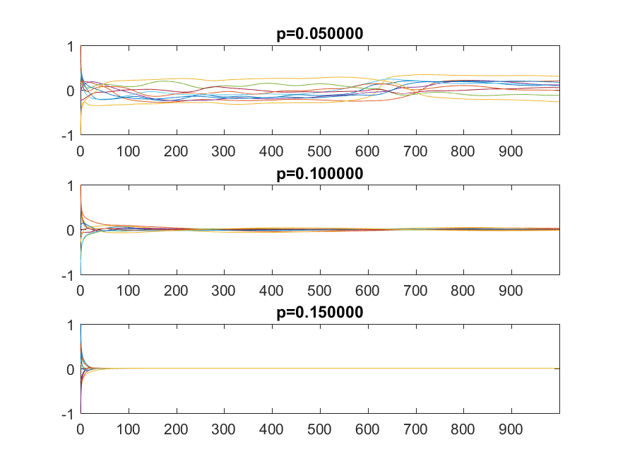
Plots of some x_i over time depending on p. The delay is=1. The top case is chaotic, the middle case is at the crossover point where the eigenvalues become negative, and the lower is beyond it.
Delay
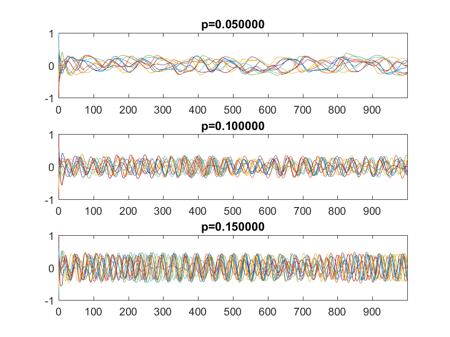
Plots of x over time depending on p, for delay=100. The top case is chaotic, becoming increasingly periodic as p increases.
But what if becomes large? In this case the force moving the trajectory towards the origin will no longer be based on where it is right now, but on where it was seconds earlier. If is small, then this is just minor noise/bias (and the dynamics is chaotic anyway). If it is large, then the trajectory will be pushed in some essentially random direction: we get instability again.
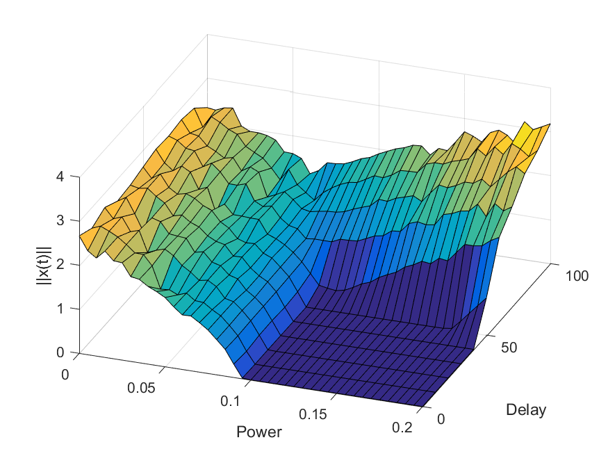
Plot of the average norm |x(t)| for some late value of t as a function of the power and delay. The dark blue square is convergence to zero, the left curved surface is chaotic motion, and the right/back surface is the delay-driven oscillations.
A (very slightly) more stringent way of thinking of it is to plug in into the equation. To simplify, let’s throw away the cubic term since we want to look at behavior close to zero, and let’s use a coordinate system where the matrix is a diagonal matrix . Then for we get , that is, the origin is a fixed point that repels or attracts trajectories depending on its eigenvalues (and we know from above that we can be pretty confident some are positive, so it is unstable overall). For we get . Taylor expansion to the first order and rearranging gives us . The numerator means that as grows, each eigenvalue will eventually get a negative real part: that particular direction of dynamics becomes stable and attracted to the origin. But the denominator can sabotage this: it gets large enough it can move the eigenvalue anywhere, causing instability.
So there you are: if you try to keep a system stable, make sure the force used is up to the task so the inherent recalcitrance cannot overwhelm it, and make sure the direction actually corresponds to the current state of the system.
 = Ax(t)/N - px(t-\tau) -x(t)^3")


||^2 x(t)")


=(2/\pi)\sqrt{1-\lambda^2}")


=c_j e^{i\lambda_j t}")


/(1 - i p \tau)")
