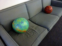
The tremendous accelerations involved in the kind of spaceflight seen on Star Trek would instantly turn the crew to chunky salsa unless there was some kind of heavy-duty protection. Hence, the inertial damping field.
— Star Trek: The Next Generation Technical Manual, page 24.
For a space opera RPG setting I am considering adding inertia manipulation technology. But can one make a self-consistent inertia dampener without breaking conservation laws? What are the physical consequences? How many cool explosions, superweapons, and other tropes can we squeeze out of it? How to avoid the worst problems brought up by the SF community?
What inertia is
As Newton put it, inertia is the resistance of an object to a change in its state of motion. Newton’s force law  is a consequence of the definition of momentum,
  (which in a way is more fundamental since it directly ties in with conservation laws). The mass in the formula is the inertial mass. Mass is a measure of how much there is of matter, and we normally multiply it with a hidden constant of 1 to get the inertial mass – this constant is what we will want to mess with.
There are relativistic versions of the laws of motion that handles momentum and inertia for high velocities, where the kinetic energy becomes so large that it starts to add mass to the whole system. This makes the total inertia go up, as seen by an outside observer, and looks like a nice case for inertia-manipulating tech being vaguely possible.
However, Einstein threw a spanner into this: gravity also acts on mass and conveniently does so exactly as much as inertia: gravitational mass (the masses in  ) and inertial mass appear to be equal. At least in my old school physics textbook (early 1980s!) this was presented as a cool unsolved mystery, but it is a consequence of the equivalence principle in general relativity (1907): all test particles accelerate the same way in a gravitational field, and this is only possible if their gravitational mass and inertial mass are proportional to one another.
So, an inertia manipulation technology will have to imply some form of gravity manipulation technology. Which may be fine from my standpoint, since what space opera is complete without antigravity? (In fact, I already had decided to have Alcubierre warp bubble FTL anyway, so gravity manipulation is in.)
Playing with inertia
OK, let’s leave relativity to the side for the time being and just consider the classical mechanics of inertia manipulation. Let us posit that there is a magical field that allows us to dial up or down the proportionality constant for inertial mass: the momentum of a particle will be  , the force law
  and the formula for kinetic energy
  \mu m v^2") .
.  is the effect of the magic field, running from
  , with 1 corresponding to it being absent.
I throw a 1 g ping-pong ball at 1 m/s into my inertics device and turn on the field. What happens? Let us assume the field is  . Now the momentum and kinetic energy jumps by a factor of 1000 if the velocity remains unchanged. Were I to catch the ball I would have gained 999 times its original kinetic energy: this looks like an excellent perpetual motion machine. Since we do not want that to be possible (a space empire powered by throwing ping-pong balls sounds silly) we must demand that energy is conserved.
Velocity shifting to preserve kinetic energy
 One way of doing energy conservation is for the velocity to go down for my heavy ping-pong ball. This means that the new velocity will be
  . Inertia-increasing fields slow down objects, while inertia-decreasing fields speed them up.
Forcefields/armour
One could have a force-field made of super-high inertia that would slow down incoming projectiles. At first this seems pointless, since once they get through to the other side they speed up and will do the same damage. But we could of course put in a bunch of armour in this field, and have it resist the projectile. The kinetic energy will be the same but it will be a lower velocity collision which means that the strength of the armour has a better chance of stopping it (in fact, as we will see below, we can use superdense armour here too). Consider the difference between being shot with a rifle bullet or being slowly but strongly stabbed by it: in the later case the force can be distributed by a good armour to a vast surface. Definitely a good thing for a space opera.
Spacecraft
A spacecraft that wants to get somewhere fast could just project a low field around itself and boost its speed by a huge  factor. Sounds very useful. But now an impacting meteorite will both have an high relative speed, and when it enters the field get that boosted by the same factor again: impacts will happen at velocities increased by a factor of
  as measured by the ship. So boosting your speed with a factor of a 1000 will give you dust hitting you at speeds a million times higher. Since typical interplanetary dust already moves a few km/s, we are talking about hyperrelativistic impactors. The armour above sounds like a good thing to have…
Note that any inertia-reducing technology is going to improve rockets even if there is no reactionless drive or other shenanigans: you just reduce the inertia of the reaction mass. The rocket equation no longer bites: sure, your ship is mostly massive reaction mass in storage, but to accelerate the ship you just take a measure of that mass, restore its inertia, expel it, and enjoy the huge acceleration as the big engine pushes the overall very low-inertia ship. There is just a snag in this particular case: when restoring the inertia you somehow need to give the mass enough kinetic energy to be at rest in relation to the ship…
Cannons
This kind of inertics does not make for a great cannon. I can certainly make my projectile speed up a lot in the bore by lowering its inertia, but as soon as it leaves it will slow down. If we assume a given amount of force  accelerating it along the length
  bore, it will pick up
  Joules of kinetic energy from the work the cannon does – independent of mass or inertia! The difference may be power: if you can only supply a certain energy per second like in a coilgun, having a slower projectile in the bore is better.
Physics
Note that entering and leaving an inertics field will induce stresses. A metal rod entering an inertia-increasing field will have the part in the field moving more slowly, pushing back against the not slowed part (yet another plus for the armour!). When leaving the field the lighter part outside will pull away strongly.
Another effect of shifting velocities is that gases behave differently. At first it looks like changing speeds would change temperature (since we tend to think of the temperature of a gas as how fast the molecules are bouncing around), but actually the kinetic temperature of a gas depends on (you guessed it) the average kinetic energy. So that doesn’t change at all. However, the speed of sound should scale as  : it becomes far higher in the inertia-dampening field, producing helium-voice like effects. Air molecules inside an inertia-decreasing field would tend to leave more quickly than outside air would enter, producing a pressure difference.
Momentum conservation is a headache
 Changing the velocity so that energy is conserved unfortunately has a drawback: momentum is not conserved! I throw a heavy object at my inertics machine at velocity
  , momentum
  and energy
 mv^2") , it reduces is inertia and increases the speed to , keeps the kinetic energy at , and the momentum is now
, it reduces is inertia and increases the speed to , keeps the kinetic energy at , and the momentum is now  .
.
What if we assume the momentum change comes from the field or machine? When I hit the mass  machine with an object it experiences a force enough to change its velocity by
 /M") . When set to increase inertia it is pushed back a bit, potentially moving up to speed
. When set to increase inertia it is pushed back a bit, potentially moving up to speed v") . When set to decrease inertia it is pushed forward, starting to move towards the direction the object impacted from. In fact, it can get arbitrarily large velocities by reducing close to 0.
. When set to decrease inertia it is pushed forward, starting to move towards the direction the object impacted from. In fact, it can get arbitrarily large velocities by reducing close to 0.
This sounds odd. Demanding momentum and energy conservation requires  (giving the above formula) and
 ^2 + Mw^2") , which insists that
, which insists that  . Clearly we cannot have both.
I don’t know about you, but I’d rather keep energy conserved. It is more obvious when you cheat about energy conservation.
Still, as Einstein pointed out using 4-vectors, momentum and energy conservation are deeply entangled – one reason inertics isn’t terribly likely in the real world is that they cannot be separated. We could of course try to conserve 4-momentum (") ), which would look like changing both energy and normal momentum at the same time.
), which would look like changing both energy and normal momentum at the same time.
Energy gain/loss to preserve momentum
 What about just retaining the normal momentum rather than the kinetic energy? The new velocity would be
  , the new kinetic energy would be
  \mu m (v/\mu)^2 = (1/2) mv^2 / \mu = K_0/\mu") . Just like in the kinetic energy preserving case the object slows down (or speeds up), but more strongly. And there is an energy debt of
. Just like in the kinetic energy preserving case the object slows down (or speeds up), but more strongly. And there is an energy debt of ") that needs to be fixed.
that needs to be fixed.
One way of resolving energy conservation is to demand that the change in energy is supplied by the inertia-manipulation device. My ping-pong ball does not change momentum, but requires 0.999 Joule to gain the new kinetic energy. The device has to provide that. When the ball leaves the field there will be a surge of energy the device needs to absorb back. Some nice potential here for things blowing up in dramatic ways, a requirement for any self-respecting space opera.
Spacecraft
If I want to accelerate my spaceship in this setting, I would point my momentum vector towards the target, reduce my inertia a lot, and then have to provide a lot of kinetic energy from my inertics devices and power supply (actually, store a lot – the energy is a surplus). At first this sounds like it is just as bad as normal rocketry, but in fact it is awesome: I can convert my electricity directly into velocity without having to lug around a lot of reaction mass! I will even get it back when slowing down, a bit like electric brake regeneration systems. The rocket equation does not apply beyond getting some initial momentum. In fact, the less velocity I have from the start, the better.
At least in this scheme inertia-reduced reaction mass can be restored to full inertia within the conceptual framework of energy addition/subtraction.
One drawback is that now when I run into interplanetary dust it will drain my batteries as the inertics system needs to give it a lot of kinetic energy (which will then go on harming me!)
Another big problem (pointed out by Erik Max Francis) is that turning energy into kinetic energy gives an energy requirement $latex dK/dt=mva$, which depends on an absolute speed. This requires a privileged reference frame, throwing out relativity theory. Oops (but not unexpected).
Forcefields/armour
Energy addition/depletion makes traditional force-fields somewhat plausible: a projectile hits the field, and we use the inertics to reduce its kinetic energy to something manageable. A rifle bullet has a few thousand Joules of energy, and if you can drain that it will now harmlessly bounce off your normal armour. Presumably shields will be depleted when the ship cannot dissipate or store the incoming kinetic energy fast enough, causing the inertics to overload and then leaving the ship unshielded.
Cannons
This kind of inertics allows us to accelerate projectiles using the inertics technology, essentially feeding them as much kinetic energy as we want. If you first make your projectile super-heavy, accelerate it strongly, and then normalise the inertia it will now speed away with a huge velocity.
Physics
A metal rod entering this kind of field will experience the same type of force as in the kinetic energy respecting model, but here the field generator will also be working on providing energy balance: in a sense it will be acting as a generator/motor. Unfortunately it does not look like it could give a net energy gain by having matter flow through.
Note that this kind of device cannot be simply turned off like the previous one: there has to be an energy accounting as everything returns to  . The really tricky case is if you are in energy-debt: you have an object of lowered inertia in the field, and cut the power. Now the object needs to get a bunch of kinetic energy from somewhere. Sudden absorption of nearby kinetic energy, freezing stuff nearby? That would break thermodynamics (I could set up a perpetual motion heat engine this way). Leaving the inertia-changed object with the changed inertia? That would mean there could be objects and particles with any effective mass – space might eventually be littered with atoms with altered inertia, becoming part of normal chemistry and physics. No such atoms have ever been found, but maybe that is because alien predecessor civilisations were careful with inertial pollution.
Other approaches
Gravity manipulation
 Another approach is to say that we are manipulating spacetime so that inertial forces are cancelled by a suitable gravity force (or, for purists, that the acceleration due to something gets cancelled by a counter-acceleration due to spacetime curvature that makes the object retain the same relative momentum).
The classic is the “gravitic drive” idea, where the spacecraft generates a gravity field somehow and then free-falls towards the destination. The acceleration can be arbitrarily large but the crew will just experience freefall. Same thing for accelerating projectiles or making force-fields: they just accelerate/decelerate projectiles a lot. Since momentum is conserved there will be recoil.
The force-fields will however be wimpy: essentially it needs to be equivalent to an acceleration bringing the projectile to a stop over a short distance. Given that normal interplanetary velocities are in tens of kilometres per second (escape velocity of Earth, more or less) the gravity field needs to be many, many Gs to work. Consider slowing down a 20 km/s railgun bullet to a stop over a distance of 10 meters: it needs to happen over a millisecond and requires a 20 million m/s^2 deceleration (2.03 megaG).
If we go with energy and momentum conservation we may still need to posit that the inertics/antigravity draws power corresponding to the work it does . Make a wheel turn because of an attracting and repulsing field, and the generator has to pay the work (plus experience a torque). Make a spacecraft go from point A to B, and it needs to pay the potential energy difference, momentum change, and at least temporarily the gain in kinetic energy. And if you demand momentum conservation for a gravitic drive, then you have the drive pulling back with the same “force” as the spacecraft experiences. Note that energy and momentum in general relativity are only locally conserved; at least this kind of drive can handwave some excuse for breaking local momentum conservation by positing that the momentum now resides in an extended gravity field (and maybe gravitational waves).
Unlike the previous kinds of inertics this doesn’t change the properties of matter, so the effects on objects discussed below do not apply.
One problem is edge tidal effects. Somewhere there is going to be a transition zone where there is a field gradient: an object passing through is going to experience some extreme shear forces and likely spaghettify. Conversely, this makes for a nifty weapon ripping apart targets.
One problem with gravity manipulation is that it normally has to occur through gravity, which is both very weak and only has positive charges. Electromagnetic technology works so well because we can play positive and negative charges against each other, getting strong effects without using (very) enormous numbers of electrons. Gravity (and gravitomagnetic effects) normally only occurs due to large mass-energy densities and momenta. So for this to work there better be antigravitons, negative mass, or some other way of making gravity behave differently from vanilla relativity. Inertics can typically handwave something about the Higgs field at least.
Forcefield manipulation
This leaves out the gravity part and just posits that you can place force vectors wherever you want. A bit like Iain M. Banks’ effector beams. No real constraints because it is entirely made-up physics; it is not clear it respects any particular conservation laws.
Other physical effects
Here are some of the nontrivial effects of changing inertia of matter (I will leave out gravity manipulation, which has more obvious effects).
Electromagnetism: beware the blue carrot
It is worth noting that this thought experiment does not affect light and other electromagnetic fields: photons are massless. The overall effect is that they will tend to push around charged objects in the field more or less. A low-inertia electron subjected to a given electric field will accelerate more, a high-inertia electron less. This in turn changes the natural frequencies of many systems: a radio antenna will change tuning depending on the inertia change. A receiver inside the inertics field will experience outside signals as being stronger (if the field decreases inertia) or weaker (if it increases it).
Reducing inertia also increases the Bohr magneton,  . This means that paramagnetic materials become more strongly affected by magnetic fields, and that ferromagnets are boosted. Conversely, higher inertia reduces magnetic effects.
Changing inertia would likely change atomic spectra (see below) and hence optical properties of many compounds. Many pigments gain their colour from absorption due to conjugated systems (think of carotene or heme) that act as antennas: inertia manipulation will change the absorbed frequencies. Carotene with increased inertia will presumably shift its absorption spectra towards lower frequencies, becoming redder, while lowered inertia causes a green or blue shift. An interesting effect is that the rhodopsin in the eye will also be affected and colour vision will experience the same shift (objects will appear to change colour in regions with a different from the place where the observer is, but not inside their field). Strong enough fields will cause shifts so that absorption and transmission outside the visual range will matter, e.g. infrared or UV becomes visible.
However, the above claim that photons should not be affected by inertia manipulation may not have to hold true. Photons carry momentum,  where k is the wave vector. So we could assume a factor of or gets in there and the field red/blueshifts photons. This would complicate things a lot, so I will leave analysis to the interested reader. But it would likely make inertics fields visible due to refractive effects.
Chemistry: toxic energy levels, plus a shrink-ray
 One area inertics would mess up is chemistry. Chemistry is basically all about the behaviour of the valence electrons of atoms. Their behaviour depends on their distribution between the atomic orbitals, which in turn depends on the Schrödinger equation for the atomic potential. And this equation has a dependency on the mass of the electron and nucleus.
If we look at hydrogen-like atoms, the main effect is that the energy levels become
") ,
,
where ") is the reduced mass. In short, the inertial manipulation field scales the energy levels up and down proportionally. One effect is that it becomes much easier to ionise low-inertia materials, and that materials that are normally held together by ionization bonds (say NaCl salt) may spontaneously decay when in high-inertia fields.
is the reduced mass. In short, the inertial manipulation field scales the energy levels up and down proportionally. One effect is that it becomes much easier to ionise low-inertia materials, and that materials that are normally held together by ionization bonds (say NaCl salt) may spontaneously decay when in high-inertia fields.
The Bohr radius scales as  : low-inertia atoms become larger. This really messes with materials. Placed in a low-inertia field atoms expand, making objects such as metals inflate. In a high inertia-field, electrons keep closer to the nuclei and objects shrink.
As distances change, the effects of electromagnetic forces also change: internal molecular electric forces, van der Waals forces and things like that change in strength, which will no doubt have effects on biology. Not to mention melting points: reducing the inertia will make many materials melt at far lower temperatures due to larger inter-atomic and inter-molecular distances, increasing it can make room-temperature liquids freeze because they are now more closely packed.
This size change also affects the electron-electron interactions, which among other things shield the nucleus and reduce the effective nuclear charge. The changed energy levels do not strongly affect the structure of the lightest atoms, so they will likely form the same kind of chemical bonds and have the same chemistry. However, heavier atoms such as copper, chromium and palladium already have ordering rules that are slightly off because of the quirks of the energy levels. As the field deviates from 1 we should expect lighter and lighter atoms to get alternative filling patterns and this means they will get different chemistry. Given that copper and chromium are essential for some enzymes, this does not bode well – if copper no longer works in cytochrome oxidase, the respiratory chain will lethally crash.
If we allow permanently inertia-altered particles chemistry can get extremely weird. An inertia-changed electron would orbit in a different way than a normal one, giving the atom it resided in entirely different chemical properties. Each changed electron could have its own individual inertia. Presumably such particles would randomise chemistry where they resided, causing all sorts of odd reactions and compounds not normally seen. The overall effect would likely be pretty toxic, since it would on average tend to catalyze metastable high-energy, low-entropy structures in biochemistry to fall down to lower energy, higher entropy states.
Lowering inertia in many ways looks like heating up things: particles move faster, chemicals diffuse more, and things melt. Given that much of biochemistry is tremendously temperature dependent, this suggests that even slight changes of to 0.99 or 1.01 would be enough to create many of the bad effects of high fever or hypothermia, and a bit more would be directly lethal as proteins denaturate.
Fluids: I need a lie down
Inside a lowered inertia field matter responds more strongly to forces, and this means that fluids flow faster for the same pressure difference. Buoyancy cases stronger convection. For a given velocity, the inertial forces are reduced compared to the viscosity, lowering the Reynolds number and making flows more laminar. Conversely, enhanced inertia fluids are hard to get to move but at a given speed they will be more turbulent.
This will really mess up the sense of balance and likely blood flow.
Gravity: equivalent exchange
I have ignored the equivalence of inertial and gravitational mass. One way for me to get away with it is to claim that they are still equivalent, since everything occurs within some local region where my inertics field is acting: all objects get their inertial mass multiplied by and this also changes their gravitational mass. The equivalence principle still holds.
What if there is no equivalence principle? I could make 1 kg object and a 1 gram object fall at different accelerations. If I had a massless spring between them it would be extended, and I would gain energy. Beside the work done by gravity to bring down the objects (which I could collect and use to put them back where they started) I would now have extra energy – aha, another perpetual motion machine! So we better stick to the equivalence principle.
Given that boosting inertia makes matter both tend to shrink to denser states and have more gravitational force, an important worldbuilding issue is how far I will let this process go. Using it to help fission or fusion seems fine. Allowing it to squeeze matter into degenerate states or neutronium might be more world-changing. And easy making of black holes is likely incompatible with the survival of civilisation.
[ Still, destroying planets with small black holes is harder than it looks. The traditional “everything gets sucked down into the singularity” scenario is surprisingly slow. If you model it using spherical Bondi accretion you need an Earth-mass black hole to make the sun implode within a year or so, and a  kg asteroid mass black hole to implode the Earth. And the extreme luminosity slows things a lot more. A better way may be to use an evaporating black hole to irradiate the solar system instead, or blow up something sending big fragments. ]
Another fun use of inertics is of course to mess up stars directly. This does not work with the energy addition/depletion model, but the velocity change model would allow creating a region of increased inertia where density ramps up: plasma enters the volume and may start descending below the spot. Conversely, reducing inertia may open a channel where it is easier for plasma from the interior to ascend (especially since it would be lighter). Even if one cannot turn this into a black hole or trigger surface fusion, it might enable directed flares as the plasma drags electromagnetic field lines with it.
The probe was invisible on the monitor, but its effects were obvious: titanic volumes of solar plasma were sucked together into a strangely geometric sunspot. Suddenly there was a tiny glint in the middle and a shock-wave: the telemetry screens went blank.
“Seems your doomsday weapon has failed, professor. Mad science clearly has no good concept of proper workmanship.”
“Stay your tongue. This is mad engineering: the energy ran out exactly when I had planned. Just watch.”
Without the probe sucking it together the dense plasma was now wildly expanding. As it expanded it cooled. Beyond a certain point it became too cold to remain plasma: there was a bright flash as the protons and electrons recombined and the vortex became transparent. Suddenly neutral the matter no longer constrained the tortured magnetic field lines and they snapped together at the speed of light. The monitor crashed.
“I really hope there is no civilization in this solar system sensitive to massive electromagnetic pulses” the professor gloated in the dark.
Conclusions
| Model |
Pros |
Cons |
| Preserve kinetic energy |
Nice armour. Fast spacecraft with no energy needs (but weird momentum changes). |
Interplanetary dust is a problem. Inertics cannons inefficient. Toxic effects on biochemistry. |
| Preserve momentum |
Nice classical forcefield. Fast spacecraft with energy demands. Inertics cannons work. Potential for cool explosions due to overloads. |
Interplanetary dust drains batteries. Extremely weird issues of energy-debts: either breaking thermodynamics or getting altered inertia materials. Toxic effects on biochemistry. Breaks relativity. |
| Gravity manipulation |
No toxic chemistry effects. Fast spacecraft with energy demands. Inertics cannons work. |
Forcefields wimpy. Gravitic drives are iffy due to momentum conservation (and are WMDs). Gravity is more obviously hard to manipulate than inertia. Tidal edge forces. |
In both cases where actual inertia is changed inertics fields appear pretty lethal. A brief brush with a weak field will likely just be incapacitating, but prolonged exposure is definitely going to kill. And extreme fields are going to do very nasty stuff to most normal materials – making them expand or contract, melt, change chemical structure and whatnot. Hence spacecraft, cannons and other devices using inertics need to be designed to handle these effects. One might imagine placing the crew compartment in a counter-inertics field keeping while the bulk of the spacecraft is surrounded by other fields. A failure of this counter-inertics field does not just instantly turn the crew into tuna paste, but into blue toxic tuna paste.
Gravity manipulation is cleaner, but this is not necessarily a plus from the cool fiction perspective: sometimes bad side effects are exactly what world-building needs. I love the idea of inertics with potential as an anti-personnel or assassination weapon through its biochemical effects, or “forcefields” being super-dense metal with amplified inertia protecting against high-velocity or beam impact.
The atomic rocket page makes a big deal out of how reactionless propulsion makes space opera destroying weapons of mass destruction (if every tramp freighter can be turned into a relativistic missile, how long is the Imperial Capital going to last?) This is a smaller problem here: being hit by a inertia-reduced freighter hurts less, even when it is very fast (think of being hit by a fast ping-pong ball). Gravity propulsion still enables some nasty relativistic weaponry, and if you spend time adding kinetic energy to your inertia-reduced missile it can become pretty nasty. But even if the reactionless aspect does not trivially produce WMDs inertia manipulation will produce a fair number of other risky possibilities. However, given that even a normal space freighter is a hypervelocity missile, the problem lies more in how to conceptualise a civilisation that regularly handles high-energy objects in the vicinity of centres of civilisation.
Not discussed here are issues of how big the fields can be made. Could we reduce the inertia of an asteroid or planet, sending it careening around? That has some big effects on the setting. Similarly, how small can we make the inertics: do they require a starship to power them, or could we have them in epaulettes? Can they be counteracted by another field?
Inertia-changing devices are really tricky to get to work consistently; most space opera SF using them just conveniently ignores the mess – just like how FTL gives rise to time travel or that talking droids ought to transform the global economy totally.
But it is fun to think through the awkward aspects, since some of them make the world-building more exciting. Plus, I would rather discover them before my players, so I can make official handwaves of why they don’t matter if they are brought up.


.}")


^{3/4} \sim 10^{27}")


^{3/4}\beta^{3/4} \sim \alpha_G^{-3/4}\times(\text{atomic factors}),")


^{3/4} \sim \alpha_G^{-3/4}\times(\text{chemistry + convention factors}) \sim 10^{24}.}")


![[3/4, 1]](http://s0.wp.com/latex.php?latex=%5B3%2F4%2C+1%5D&bg=ffffff&fg=000000&s=0 "[3/4, 1]")


^{4}")


 . Sure, dipoles and multipoles may add higher order terms, and extended conductors like wires and planes produce other behaviour. But most of us think we can trust the
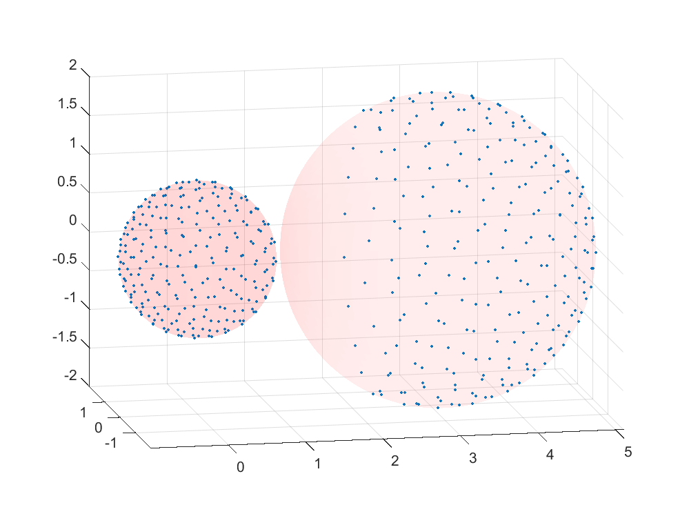
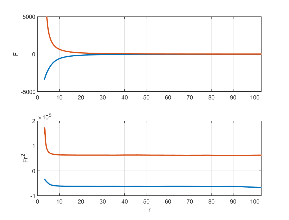
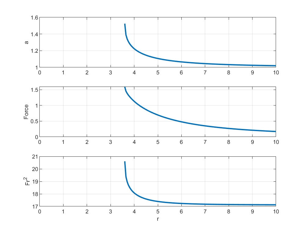
=-GM/r") potential as
potential as =-GM/(r-R_S)") (where
(where  is the Schwarzschild radius). It makes the force increase faster than the classical potential as we approach
  .
.
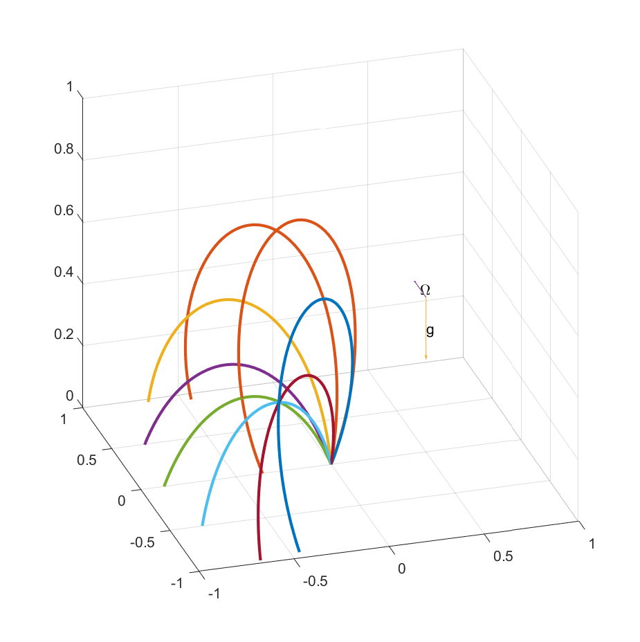
") ) and release particles from different locations they will swing around the masses in some trajectory. If we colour each point by the mass it approaches closest (or even collides with) we get a basin of attraction for each mass. Can one prove the boundary is a straight line?
) and release particles from different locations they will swing around the masses in some trajectory. If we colour each point by the mass it approaches closest (or even collides with) we get a basin of attraction for each mass. Can one prove the boundary is a straight line? around the masses. Dark regions take long to approach any of the masses, white regions don’t converge within a given cut-off time.
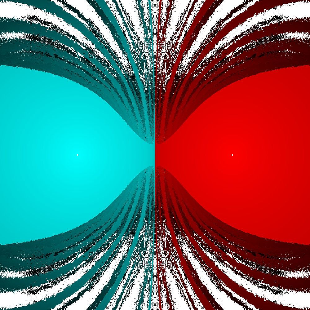
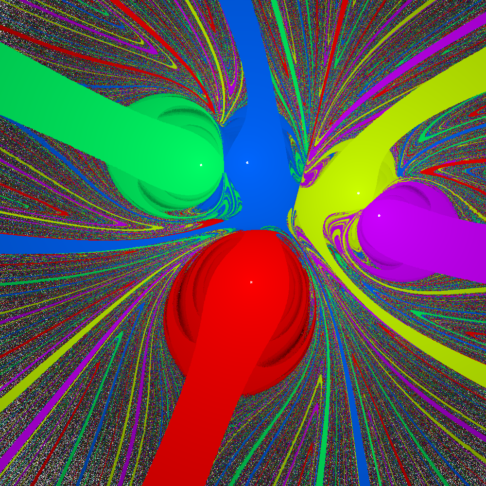
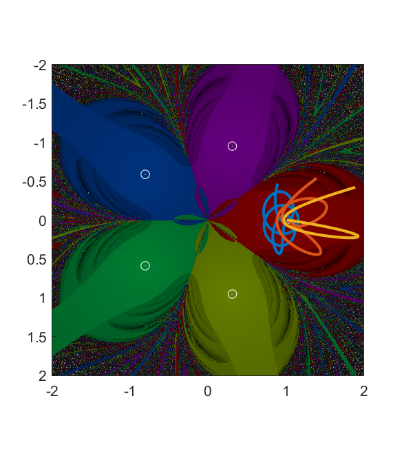
 and 0.01 (assuming unit masses at unit distance from origin and
  ) is somewhat prettier.

 the basins approach ellipses around their central mass, corresponding to orbits that loop around them in elliptic orbits that eventually get close enough to count as a hit. The onion-like shading is due to different number of orbits before this happens. Each basin also has a tail or stem, corresponding to plunging orbits coming in from afar and hitting the mass straight. As the trap condition is made stricter they become thinner and thinner, yet form an ever more intricate chaotic web oughtside the central region. Due to computational limitations (read: only a laptop available) these pictures are of relatively modest integration times.
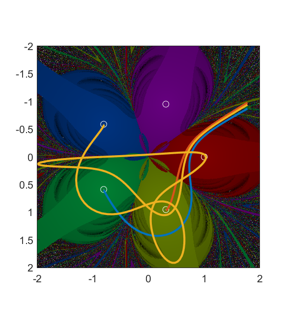
![[0,1]](http://s0.wp.com/latex.php?latex=%5B0%2C1%5D&bg=ffffff&fg=000000&s=0 "[0,1]") to
to ") that is a homeomorphism. There are hence just N basins of attraction, plus a set of unstable separatrix points that never approach the masses. Some of these border points are just invariant (like the origin in the case of the evenly distributed masses), others correspond to unstable orbits.
that is a homeomorphism. There are hence just N basins of attraction, plus a set of unstable separatrix points that never approach the masses. Some of these border points are just invariant (like the origin in the case of the evenly distributed masses), others correspond to unstable orbits. where
where ") counts the time until collision (i.e. backwards). These collision manifolds must extend through the basin of attraction, approaching the border in ever more convoluted ways as
counts the time until collision (i.e. backwards). These collision manifolds must extend through the basin of attraction, approaching the border in ever more convoluted ways as  approaches
  . Each border point has a neighbourhood where there are infinitely many trajectories directly hitting one of the masses. They form 3D sheets get stacked like an infinitely dense mille-feuille cake in the 4D phase space. And typically these sheets are interleaved with the sheets of the other attractors. The end result is very much like the
 ") force rather than the
force rather than the  .
. If we just look at the velocity vector we get
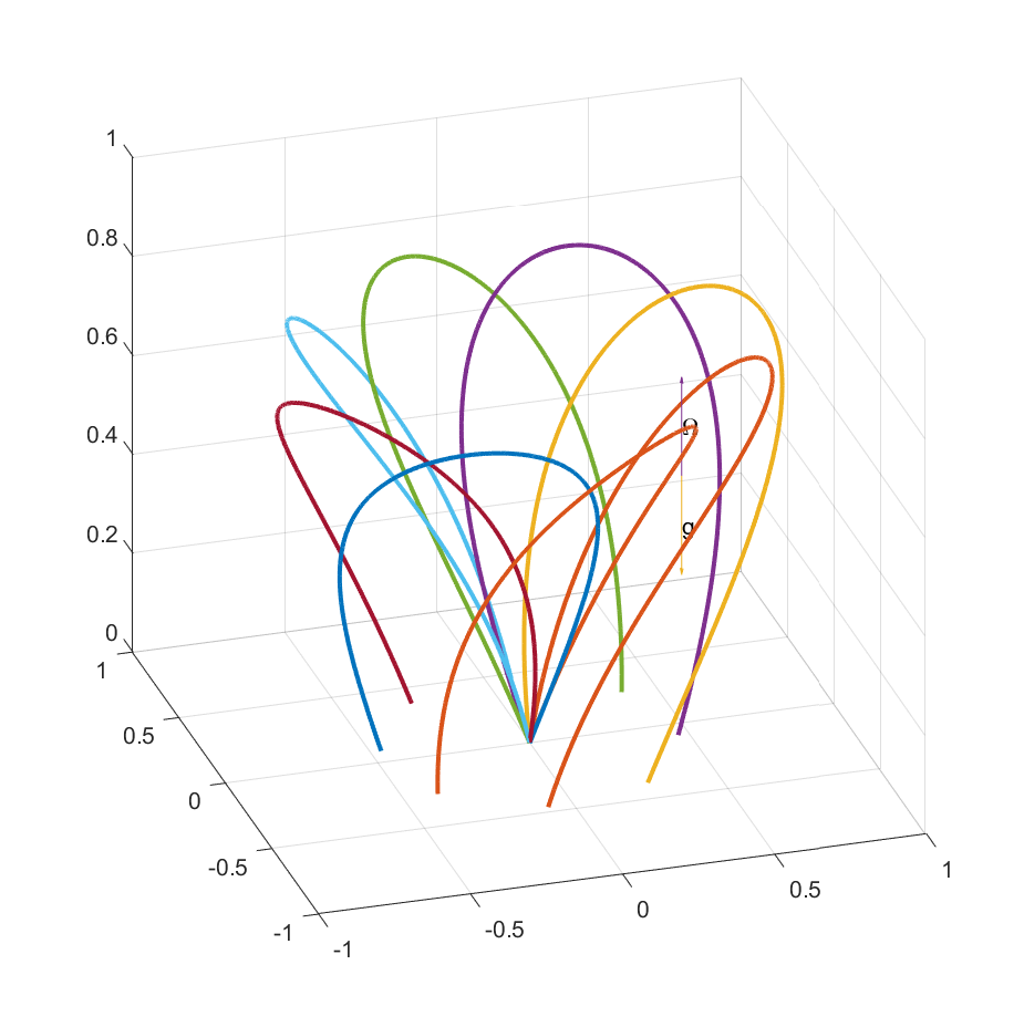
 direction. The helix radius will be
  .
. . On Donut it is 0.000614 and on Hoop 0.000494, several times higher. Still, the correction is not going to be enormous: for a ball moving 10 meters per second the helix radius will be 69 km on Earth (at the pole), 8.1 km on Donut, and 10 km on Hoop. We hence need to throw the ball a suborbital distance before the twists become really visible. At these distances the curvature of the planet and the non-linearity of the gravitational field also begins to bite.
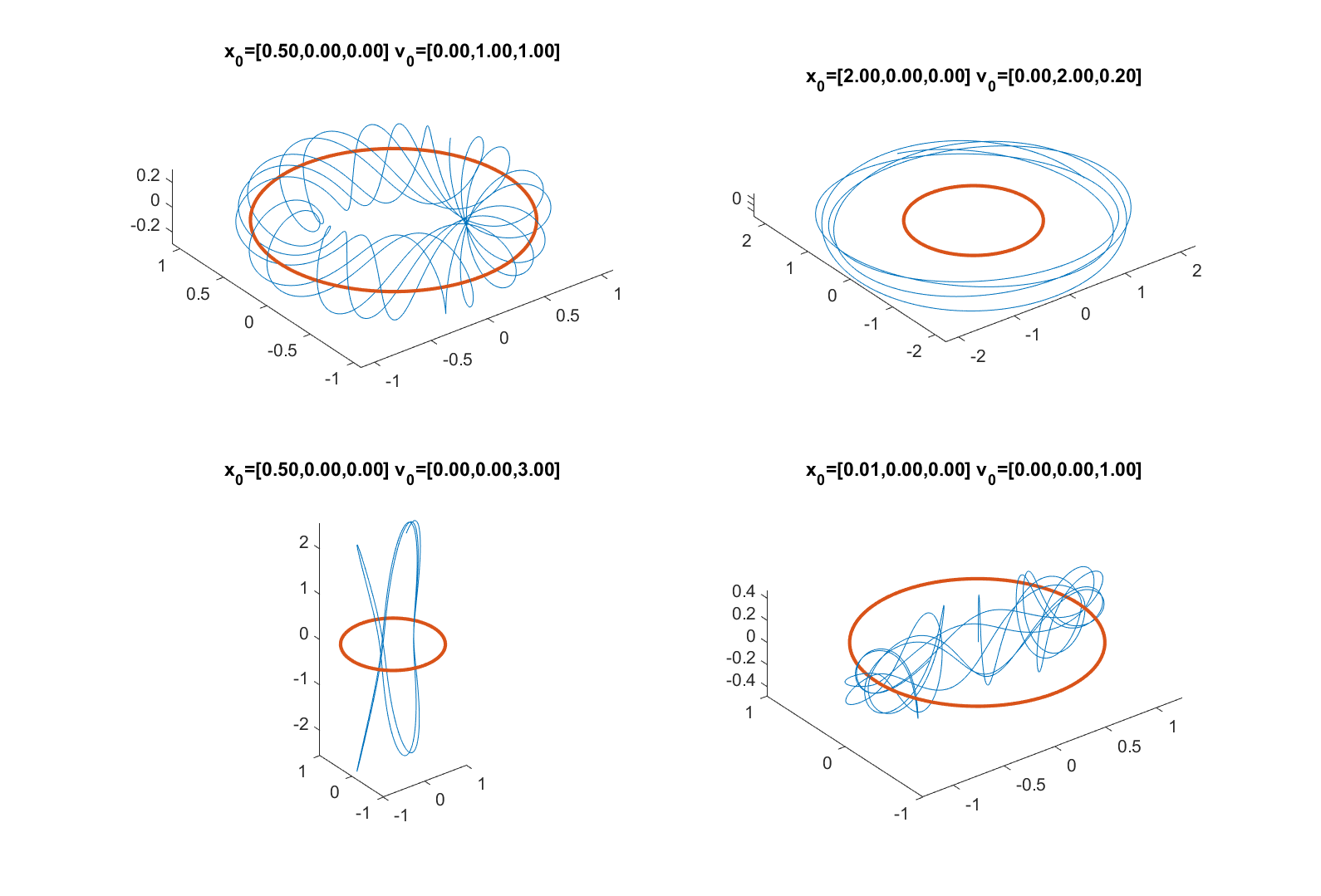

 kg/m3 appears to be reasonable.
  .
. N/m2. This allows us to estimate at what depth the berries will start to break:
  m. So while the surface will be free blueberries they will start pulping within a few meters of the surface.
 , or
, or ^{1/3}r_{earth}") . In this case we end up with a planet with 0.8879 times smaller radius (5,657 km), surrounded by a vast atmosphere.
. In this case we end up with a planet with 0.8879 times smaller radius (5,657 km), surrounded by a vast atmosphere.![\int_0^R G [4\pi r^2 \rho] [4 \pi r^3 \rho/3] / r dr](http://s0.wp.com/latex.php?latex=%5Cint_0%5ER+G+%5B4%5Cpi+r%5E2+%5Crho%5D+%5B4+%5Cpi+r%5E3+%5Crho%2F3%5D+%2F+r+dr+&bg=ffffff&fg=000000&s=0 "\int_0^R G [4\pi r^2 \rho] [4 \pi r^3 \rho/3] / r dr")
 \int_0^R r^4 dr")
\rho^2 R^5")
(\rho_{berries}^2 r_{earth}^5 - \rho_{pulp}^2R_{pulp}^5)")
 J.
J. km, about two-thirds of the radius. This would make up most of the interior. However, gravity is a bit weaker in the interior, so we need to take that into account. The pressure from all the matter above radius r is
  =(3GM^2/8\pi R^4)(1-(r/R)^2)") , and the ice core will have radius
, and the ice core will have radius }")
 3,258 km. This is smaller, about 57% of the radius, and just 20% of the total volume.
MR_1^2(2\pi/T_1) = (2/5)MR_2^2(2\pi/T_2)") , or
, or ^2 T_1") , in this case 18.9210 hours. This in turn will increase the oblateness a bit, to
, in this case 18.9210 hours. This in turn will increase the oblateness a bit, to  1.6925
  J, while the kinetic energy is
  J – more than enough to escape. Had it remained the jam ocean would have made an excellent tidal dissipation mechanism that would have slowed down rotation and moved blueberry earth towards tidal lock with the moon much earlier than the 50 billion years it would otherwise have taken.
 , and subtract the atomic number
  since that is the number of protons:
  . Now we know how many neutrons there are per atom on average (standard atomic weights include the different isotope weights, weighted by their abundance).
 kg, so the number of nucleons per kilogram is
 ") and the number of neutrons per kilo is
and the number of neutrons per kilo is ") . This ranges from
. This ranges from  for helium down to
  for Oganesson. Hydrogen just has
  neutrons per kilogram, despite having
  nucleons per kilogram – there isn’t that much deuterium and tritium around to contribute neutrons.
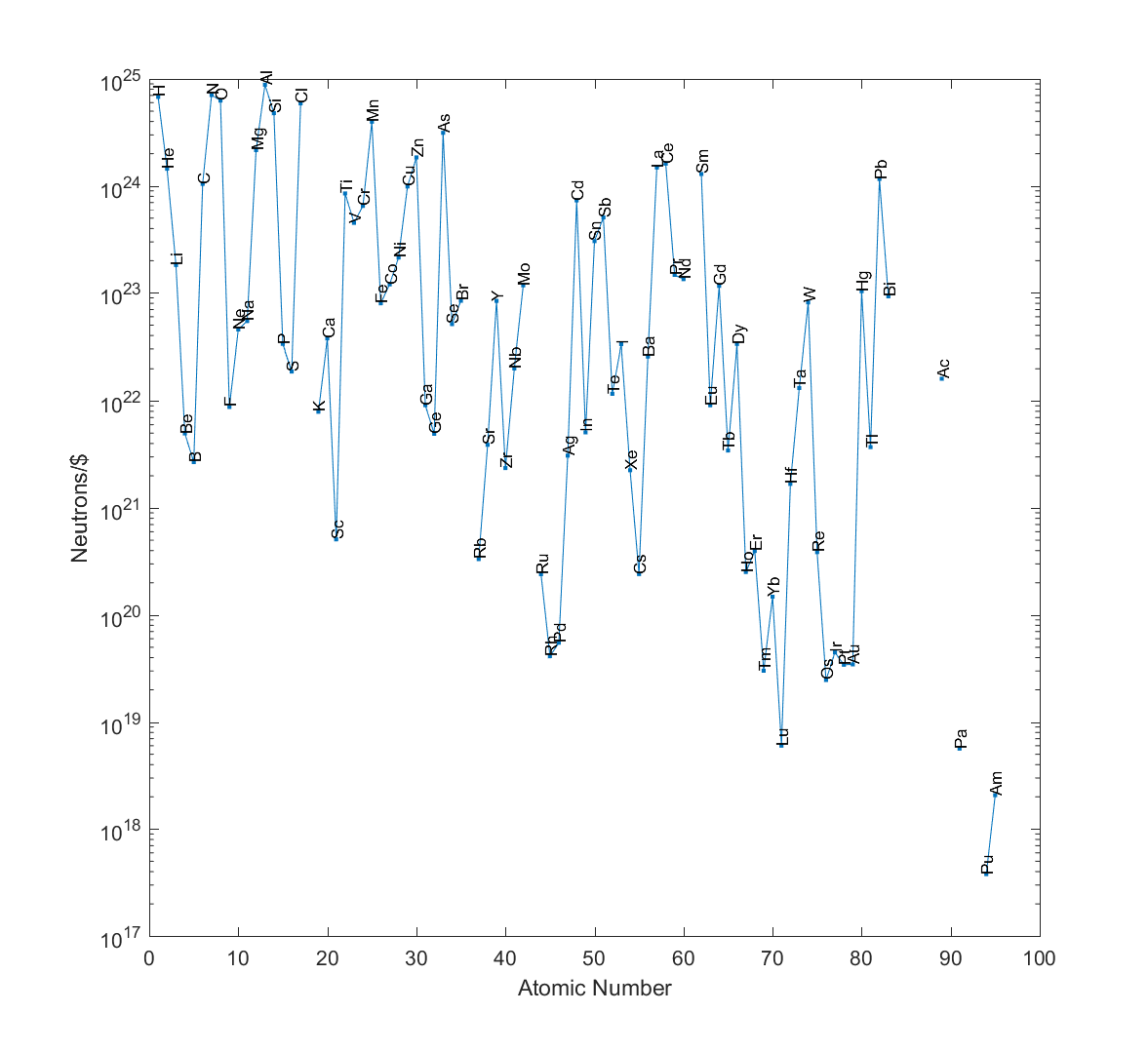
 neutrons per dollar from aluminium.
 ) and in third, hydrogen (
 )! Hydrogen may be very neutron-poor, but since it is rather cheap and you get lots of nucleons per kilo, this balances the lack.
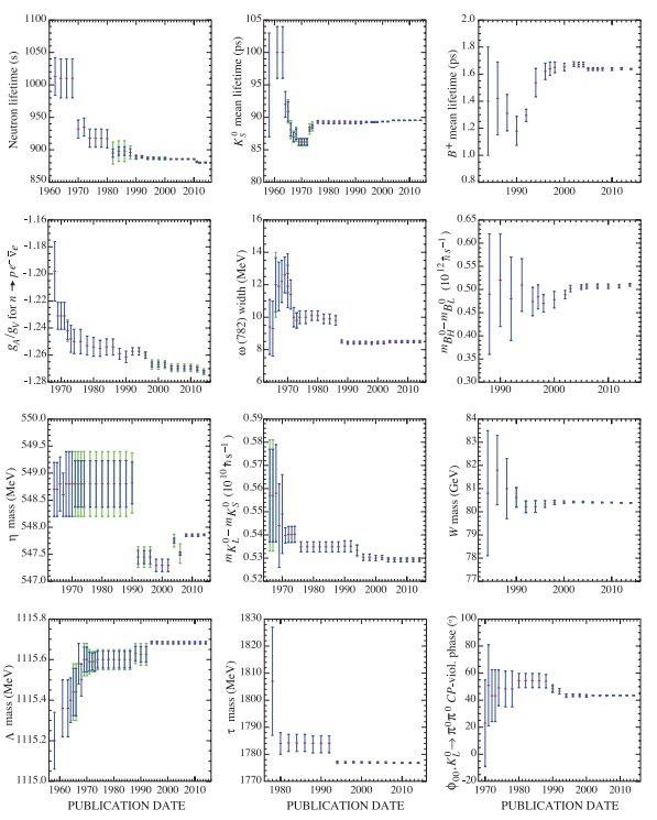
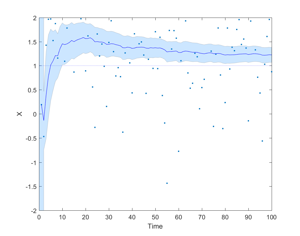
 data points and seen
  big surprises (remember that the first data point counts as one!), then the probability of a new surprise for your next data point is
  . So if you expect
 /N \ll 1") you can start to trust the estimates… assuming surprises are uncorrelated etc. Which you will not be certain about. The progression towards greater precision may be anything but dull.
you can start to trust the estimates… assuming surprises are uncorrelated etc. Which you will not be certain about. The progression towards greater precision may be anything but dull.