Apropos Newton’s method in the complex plane, what happens when the degree of the polynomial goes to infinity?

Towards infinity

Obviously there will be more zeros, so there will be more attractors and we should expect the boundaries of the basins of attraction to become messier. But it is not entirely clear where the action will be, so it would be useful to compress the entire complex plane into a convenient square.

How do you depict the entire complex plane? While I have always liked the Riemann sphere here I tried mapping to . The origin is unchanged, and infinity becomes the edges of the square . This is not a conformal map, so things will get squished near the edges.

For color, I used to map complex coordinates to RGB. This makes the color depend on the distance to 1, -1 and i, making infinity white and zero some drab color (the -1 terms at the end determines the overall color range).

Here is the animated result:

What is going on? As I scale up the size of the leading term from zero, the root created by adding that term moves in from infinity towards the center, making the new basin of attraction grow. This behavior has been described in this post on dancing zeros. The zeros also tend to cluster towards the unit circle, crowding together and distributing themselves evenly. That distribution is the reason for the the colorful “flowers” that surround white spots (poles of the Newton formula, corresponding to zeros of the derivative of the polynomial). The central blob is just the attractor of the most “solid” zero, corresponding to the linear and constant terms of the polynomial.

The jostling is amusing: it looks like the roots do repel each other. This is presumably because close roots require a sharp turn of the function, but the “turning radius” is set by the coefficients that tend to be of order unity. Getting degenerate roots requires coefficients to be in a set of measure zero, so it is rare. Near-degenerate roots exist in a positive measure set surrounding that set, but it is still “small” compared to the general case.

At infinity

So what happens if we let the degree go to infinity? As I previously mentioned, the generic behaviour of where is independent random numbers is a lacunary function. So we should not expect anything outside the unit circle. Inside the circle there will be poles, so there will be copies of the undefined outside region (because of Great Picard’s Theorem (meromorphic version)). Since the function is analytic these copies will be conformal mappings of the exterior and hence roughly circular. There will also be zeros, and these will have their own basins of attraction. A few of the central ones dominate, but there is an infinite number of attractors as we approach the circular border which is crammed with poles and zeros.

Since we now know we will only deal with the unit disk, we can avoid transforming the entire plane and enjoy the results:

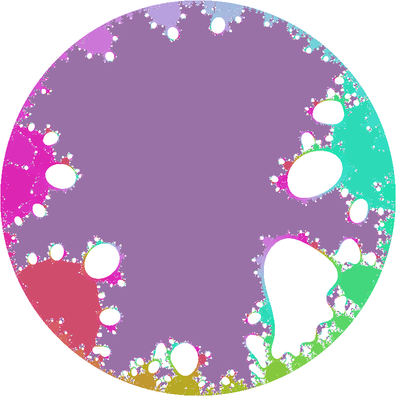
What happens here is that the white regions represents places where points get mapped onto the undefined outside, while the colored fractal regions are the attraction basins for the zeros. And between them there is a truly wild boundary. In the vanilla fractal every point on the boundary is a meeting point of the three basins, a tri-point. Here there is an infinite number of attractors: the boundary consists of points where an infinite number of different attractors meet.