It is Newtonmass, and that means doing some fun math. I try to invent a new fractal or something similar every year: this is the result for 2018.
The Newton fractal is an old classic. Newton’s method for root finding iterates an initial guess to find a better approximation . This will work as long as , but which root one converges to can be sensitively dependent on initial conditions. Plotting which root a given initial value ends up with gives the Newton fractal.
The Newton-Gauss method is a method for minimizing the total squared residuals when some function dependent on n-dimensional parameters $\beta$ is fitted to data points . Just like the root finding method it iterates towards a minimum of : where is the Jacobian . This is essentially Newton’s method but in a multi-dimensional form.
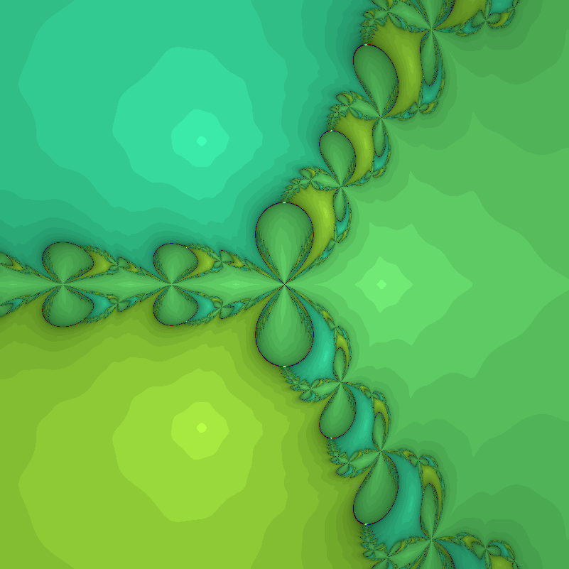
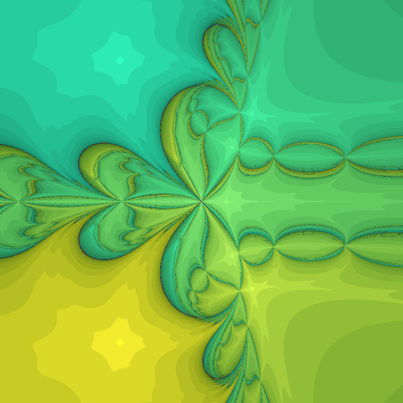
So we can make fractals by trying to fit (say) a function consisting of the sum of two Gaussians with different means (but fixed variances) to a random set of points. So we can set (one Gaussian with variance 1 and one with 1/4 – the reason for this is not to make the diagram boringly symmetric as for the same variance case). Plotting the location of the final (by stereographically mapping it onto a unit sphere in (r,g,b) space) gives a nice fractal:
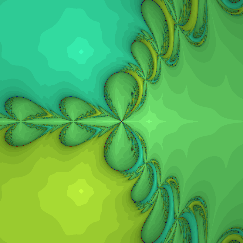
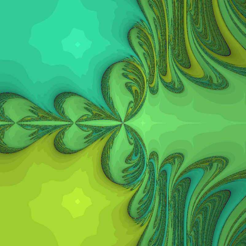
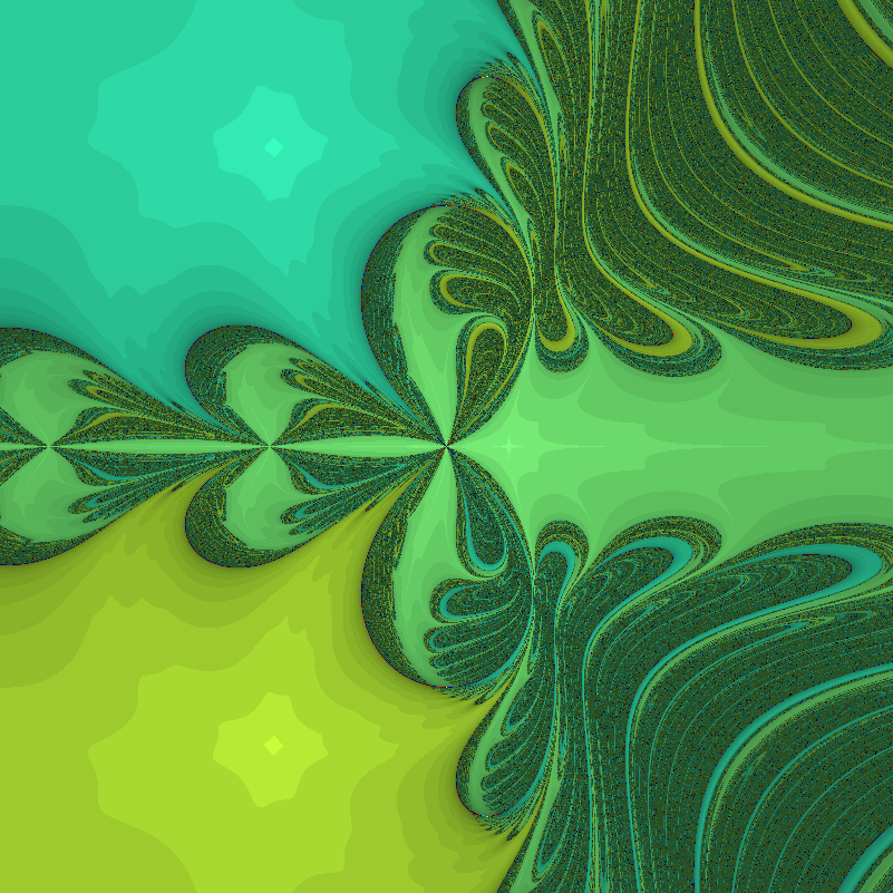
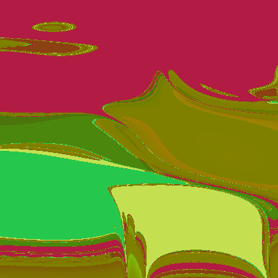
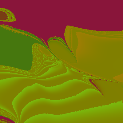
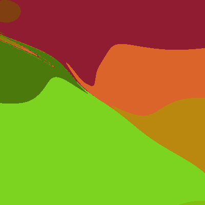
Basins of attraction of different attractor states of Gauss-Newton’s method. Two Gaussian functions fitted to five random points.Basins of attraction of different attractor states of Gauss-Newton’s method. Two Gaussian functions fitted to 10 random points.Basins of attraction of different attractor states of Gauss-Newton’s method. Two Gaussian functions fitted to 50 random points.
It is a bit modernistic-looking. As I argued in 2016, this is because the generic local Jacobian of the dynamics doesn’t have much rotation.
As more and more points are added the attractor landscape becomes simpler, since it is hard for the Gaussians to “stick” to some particular clump of points and the gradients become steeper.
This fractal can obviously be generalized to more dimensions by using more parameters for the Gaussians, or more Gaussians etc.
The fractality is guaranteed by the generic property of systems with several attractors that points at the border of two basins of attraction will tend to find their ways to other attractors than the two equally balanced neighbors. Hence a cut transversally across the border will find a Cantor-set of true basin boundary points (corresponding to points that eventually get mapped to a singular Jacobian in the iteration formula, like the boundary of the Newton fractal is marked by points mapped to for some n) with different basins alternating.
Apropos Newton’s method in the complex plane, what happens when the degree of the polynomial goes to infinity?
Towards infinity
Obviously there will be more zeros, so there will be more attractors and we should expect the boundaries of the basins of attraction to become messier. But it is not entirely clear where the action will be, so it would be useful to compress the entire complex plane into a convenient square.
How do you depict the entire complex plane? While I have always liked the Riemann sphere here I tried mapping to . The origin is unchanged, and infinity becomes the edges of the square . This is not a conformal map, so things will get squished near the edges.
For color, I used to map complex coordinates to RGB. This makes the color depend on the distance to 1, -1 and i, making infinity white and zero some drab color (the -1 terms at the end determines the overall color range).
Here is the animated result:
What is going on? As I scale up the size of the leading term from zero, the root created by adding that term moves in from infinity towards the center, making the new basin of attraction grow. This behavior has been described in this post on dancing zeros. The zeros also tend to cluster towards the unit circle, crowding together and distributing themselves evenly. That distribution is the reason for the the colorful “flowers” that surround white spots (poles of the Newton formula, corresponding to zeros of the derivative of the polynomial). The central blob is just the attractor of the most “solid” zero, corresponding to the linear and constant terms of the polynomial.
The jostling is amusing: it looks like the roots do repel each other. This is presumably because close roots require a sharp turn of the function, but the “turning radius” is set by the coefficients that tend to be of order unity. Getting degenerate roots requires coefficients to be in a set of measure zero, so it is rare. Near-degenerate roots exist in a positive measure set surrounding that set, but it is still “small” compared to the general case.
At infinity
So what happens if we let the degree go to infinity? As I previously mentioned, the generic behaviour of where is independent random numbers is a lacunary function. So we should not expect anything outside the unit circle. Inside the circle there will be poles, so there will be copies of the undefined outside region (because of Great Picard’s Theorem (meromorphic version)). Since the function is analytic these copies will be conformal mappings of the exterior and hence roughly circular. There will also be zeros, and these will have their own basins of attraction. A few of the central ones dominate, but there is an infinite number of attractors as we approach the circular border which is crammed with poles and zeros.
Since we now know we will only deal with the unit disk, we can avoid transforming the entire plane and enjoy the results:
Attractors for random 10,000-degree polynomial.Attractors for random 10,000-degree polynomial.
What happens here is that the white regions represents places where points get mapped onto the undefined outside, while the colored fractal regions are the attraction basins for the zeros. And between them there is a truly wild boundary. In the vanilla fractal every point on the boundary is a meeting point of the three basins, a tri-point. Here there is an infinite number of attractors: the boundary consists of points where an infinite number of different attractors meet.
But what if we looked at real functions? If we use a single function the zeros will typically form a curve in the plane. In order to get discrete zeros we typically need to have two functions to produce a zero set. We can think of it as a map from R2 to R2 where the x’es are 2D vectors. In this case Newton’s method turns into solving the linear equation system where is the Jacobian matrix () and now denotes the n’th iterate.
The simplest case of nontrivial dynamics of the method is for third degree polynomials, and we want the x- and y-directions to interact a bit, so a first try is . Below is a plot of the first and second components (red and green), as well as a blue plane for zero values. The zeros of the function are the three points where red, green and blue meet.
We have three zeros, one at , one at , and one at The middle one has a region of troublesomely similar function values – the red and green surfaces are tangent there.
Plot of x^3-x-y (red), y^3-x-y (green) and z=0 (blue). The zeros found using Newton’s method are the points where red, green and blue meet.
The resulting fractal has a decided modernist bent to it, all hyperbolae and swooshes:
Behavior of Newton’s method in 2D for F=[x^3-x-y, y^3-x-y]. Color denotes value of x+y, with darkening for slow convergence.The troublesome region shows up, as well as the red and blue regions where iterates run off to large or small values: the three roots are green shades.
Why is the style modernist?
In complex iterations you typically multiply with complex numbers, and if they have an imaginary component (they better have, to be complex!) that introduces a rotation or twist. Hence baroque filaments are ubiquitous, and you get the typical complex “style”.
But here we are essentially multiplying with a real matrix. For a real 2×2 matrix to be a rotation matrix it has to have a pair of imaginary eigenvalues, and for it to at least twist things around the trace needs to be small enough compared to the determinant so that there are complex eigenvalues: (where and if the matrix has the usual form). So if the trace and determinant are randomly chosen, we should expect a majority of cases to be non-rotational.
Moreover, in this particular case, the Jacobian tends to be diagonally dominant (quadratic terms on the diagonal) and that makes the inverse diagonally dominant too: the trace will be big, and hence the chance of seeing rotation goes down even more. The two “knots” where a lot of basins of attraction come together are the points where the trace does vanish, but since the Jacobian is also symmetric there will not be any rotation anyway. Double guarantee.
Can we make a twisty real Newton fractal? If we start with a vanilla rotation matrix and try to find a function that produces it the simplest case is . This is of course just a rotation by the angle theta, and it does not have very interesting zeros.
To get something fractal we need more zeros, and a few zeros in the derivatives too (why? because they cause iterates to be thrown away far from where they were, ensuring a complicated structure of the basin boundaries). One attempt is . The result is fun, but still far from baroque:
Basins of attraction for Netwon’s method of twisted cubic. theta=1.Basins of attraction for Netwon’s method of twisted cubic. theta=0.1.
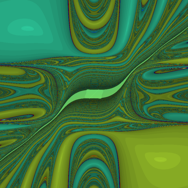
The problem might be that the twistiness is not changing. So we can make to make the dynamics even more complex:
Basins of attraction with rotation proportional to x.
Quite lovely, although still not exactly what I wanted (sounds like a Christmas present).
Back to the classics?
It might be easier just to hide the complex dynamics in an apparently real function like (which produces the archetypal Newton fractal).
Newton fractal for F=[x^3-3xy^2-1, 3x^2y-y^3]. Red and blue circles mark regions where iterates venture far from the origin.It is interesting to see how much perturbing it causes a modernist shift. If we use , then for we get:
Perturbed z^3-1 Newton iteration, epsilon=1.
As we make the function more perturbed, it turns more modernist, undergoing a topological crisis for epsilon between 3.5 and 4:
Perturbed z^3-1 Newton iteration, epsilon=2.Perturbed z^3-1 Newton iteration, epsilon=3.Perturbed z^3-1 Newton iteration, epsilon=3.5.Perturbed z^3-1 Newton iteration, epsilon=4.
In the end, we can see that the border between classic baroque complex fractals and the modernist swooshy real fractals is fuzzy. Or, indeed, fractal.

/f'(z_{n})")
\neq 0")
=\sum_{i=1}^m r_i^2(\beta)")

=f(x_i;\beta)-y_i")
")
^{-1}J^t r(\beta)")


![f(x;\beta_1,\beta_2)=(1/\sqrt{2\pi})[e^{-(x-\beta_1)^2/2}+(1/4)e^{-(x-\beta_1)^2/8}]](http://s0.wp.com/latex.php?latex=f%28x%3B%5Cbeta_1%2C%5Cbeta_2%29%3D%281%2F%5Csqrt%7B2%5Cpi%7D%29%5Be%5E%7B-%28x-%5Cbeta_1%29%5E2%2F2%7D%2B%281%2F4%29e%5E%7B-%28x-%5Cbeta_1%29%5E2%2F8%7D%5D&bg=ffffff&fg=000000&s=0 "f(x;\beta_1,\beta_2)=(1/\sqrt{2\pi})[e^{-(x-\beta_1)^2/2}+(1/4)e^{-(x-\beta_1)^2/8}]")
")
=0")
 to
to ![[\tanh(x),\tanh(y)]](http://s0.wp.com/latex.php?latex=%5B%5Ctanh%28x%29%2C%5Ctanh%28y%29%5D&bg=ffffff&fg=000000&s=0 "[\tanh(x),\tanh(y)]") . The origin is unchanged, and infinity becomes the edges of the square
. The origin is unchanged, and infinity becomes the edges of the square ![[-1,1]\times [-1,1]](http://s0.wp.com/latex.php?latex=%5B-1%2C1%5D%5Ctimes+%5B-1%2C1%5D&bg=ffffff&fg=000000&s=0 "[-1,1]\times [-1,1]") . This is not a conformal map, so things will get squished near the edges.
. This is not a conformal map, so things will get squished near the edges.![(1/2)+(1/2)[\tanh(|z-1|-1), \tanh(|z+1|-1), \tanh(|z-i|-1)]](http://s0.wp.com/latex.php?latex=%281%2F2%29%2B%281%2F2%29%5B%5Ctanh%28%7Cz-1%7C-1%29%2C+%5Ctanh%28%7Cz%2B1%7C-1%29%2C+%5Ctanh%28%7Cz-i%7C-1%29%5D&bg=ffffff&fg=000000&s=0 "(1/2)+(1/2)[\tanh(|z-1|-1), \tanh(|z+1|-1), \tanh(|z-i|-1)]") to map complex coordinates to RGB. This makes the color depend on the distance to 1, -1 and i, making infinity white and zero some drab color (the -1 terms at the end determines the overall color range).
to map complex coordinates to RGB. This makes the color depend on the distance to 1, -1 and i, making infinity white and zero some drab color (the -1 terms at the end determines the overall color range). where
where  is independent random numbers is a

 fractal every point on the boundary is a meeting point of the three basins, a
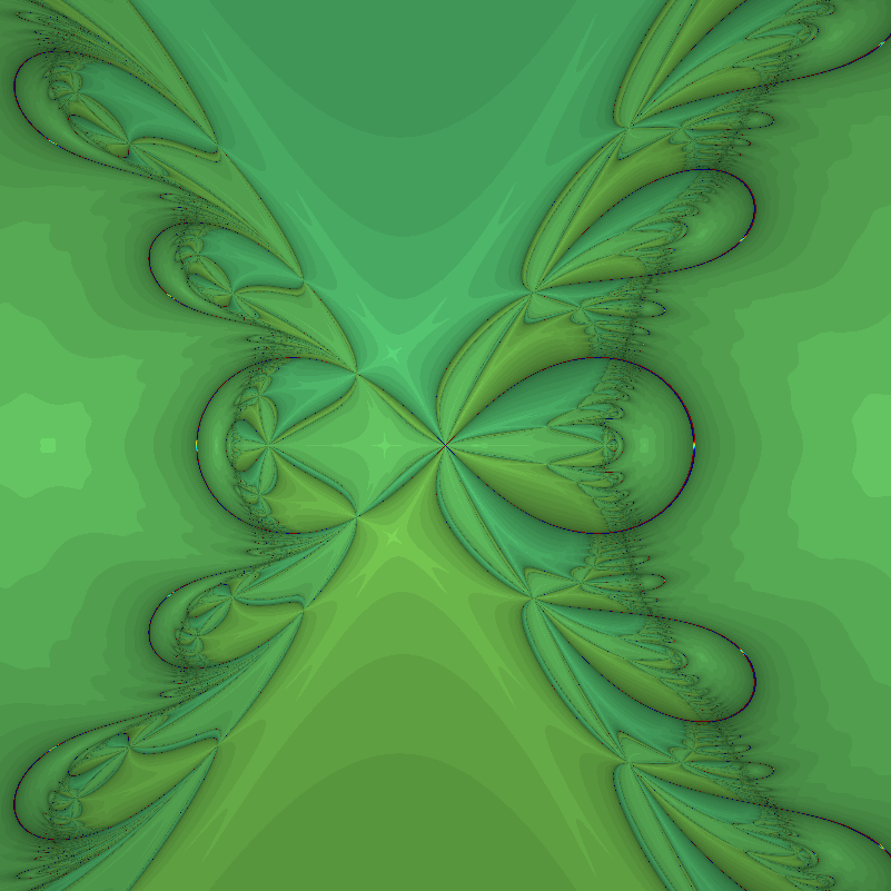
") the zeros will typically form a curve in the plane. In order to get discrete zeros we typically need to have two functions to produce a zero set. We can think of it as a map from R2 to R2
the zeros will typically form a curve in the plane. In order to get discrete zeros we typically need to have two functions to produce a zero set. We can think of it as a map from R2 to R2 ![F(x)=[f_1(x_1,x_2), f_2(x_1,x_2)]](http://s0.wp.com/latex.php?latex=F%28x%29%3D%5Bf_1%28x_1%2Cx_2%29%2C+f_2%28x_1%2Cx_2%29%5D+&bg=ffffff&fg=000000&s=0 "F(x)=[f_1(x_1,x_2), f_2(x_1,x_2)]") where the x’es are 2D vectors. In this case Newton’s method turns into solving the linear equation system
where the x’es are 2D vectors. In this case Newton’s method turns into solving the linear equation system (x_{n+1}-x_n)=-F(x_n)") where
where ") is the Jacobian matrix (
is the Jacobian matrix ( ) and
) and  now denotes the n’th iterate.
![F=[x^3-x-y, y^3-x-y]](http://s0.wp.com/latex.php?latex=F%3D%5Bx%5E3-x-y%2C+y%5E3-x-y%5D&bg=ffffff&fg=000000&s=0 "F=[x^3-x-y, y^3-x-y]") . Below is a plot of the first and second components (red and green), as well as a blue plane for zero values. The zeros of the function are the three points where red, green and blue meet.
. Below is a plot of the first and second components (red and green), as well as a blue plane for zero values. The zeros of the function are the three points where red, green and blue meet. , one at
  , and one at
  The middle one has a region of troublesomely similar function values – the red and green surfaces are tangent there.
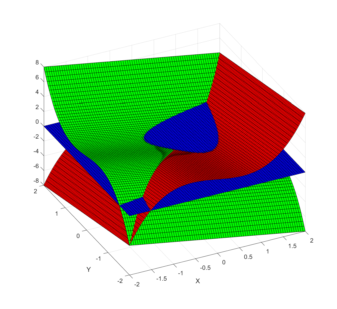
![Behavior of Newton's method in 2D for F=[x^3-x-y, y^3-x-y]. Color denotes value of x+y, with darkening for slow convergence.](http://aleph.se/andart2/wp-content/uploads/2016/12/newton2dp1.png)
 (where
  and
and  if the matrix has the usual
 ![[a b; c d]](http://s0.wp.com/latex.php?latex=%5Ba+b%3B+c+d%5D&bg=ffffff&fg=000000&s=0 "[a b; c d]") form). So if the trace and determinant are randomly chosen, we should expect a majority of cases to be non-rotational.
form). So if the trace and determinant are randomly chosen, we should expect a majority of cases to be non-rotational.![F=[x \cos(\theta) + y \sin(\theta), x\sin(\theta)+y\cos(\theta)]](http://s0.wp.com/latex.php?latex=F%3D%5Bx+%5Ccos%28%5Ctheta%29+%2B+y+%5Csin%28%5Ctheta%29%2C+x%5Csin%28%5Ctheta%29%2By%5Ccos%28%5Ctheta%29%5D&bg=ffffff&fg=000000&s=0 "F=[x \cos(\theta) + y \sin(\theta), x\sin(\theta)+y\cos(\theta)]") . This is of course just a rotation by the angle theta, and it does not have very interesting zeros.
. This is of course just a rotation by the angle theta, and it does not have very interesting zeros. \cos(\theta)")
 \sin(\theta),")
![(x^3-x-y) \sin(\theta)+(y^3-y-x) \cos(\theta) ]](http://s0.wp.com/latex.php?latex=%28x%5E3-x-y%29+%5Csin%28%5Ctheta%29%2B%28y%5E3-y-x%29+%5Ccos%28%5Ctheta%29+%5D&bg=ffffff&fg=000000&s=0 "(x^3-x-y) \sin(\theta)+(y^3-y-x) \cos(\theta) ]") . The result is fun, but still far from baroque:
. The result is fun, but still far from baroque: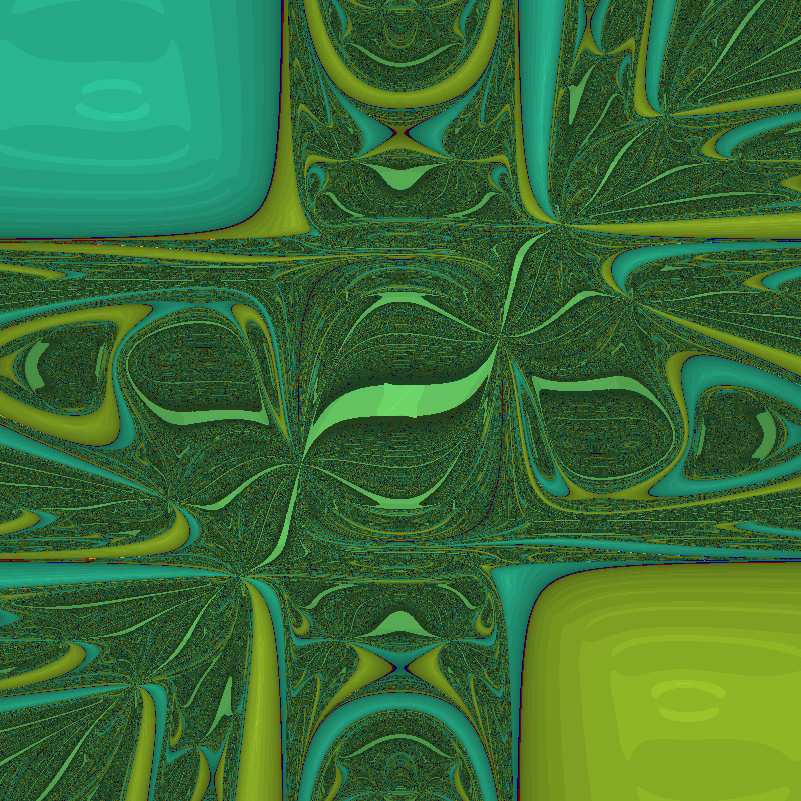
 to make the dynamics even more complex:
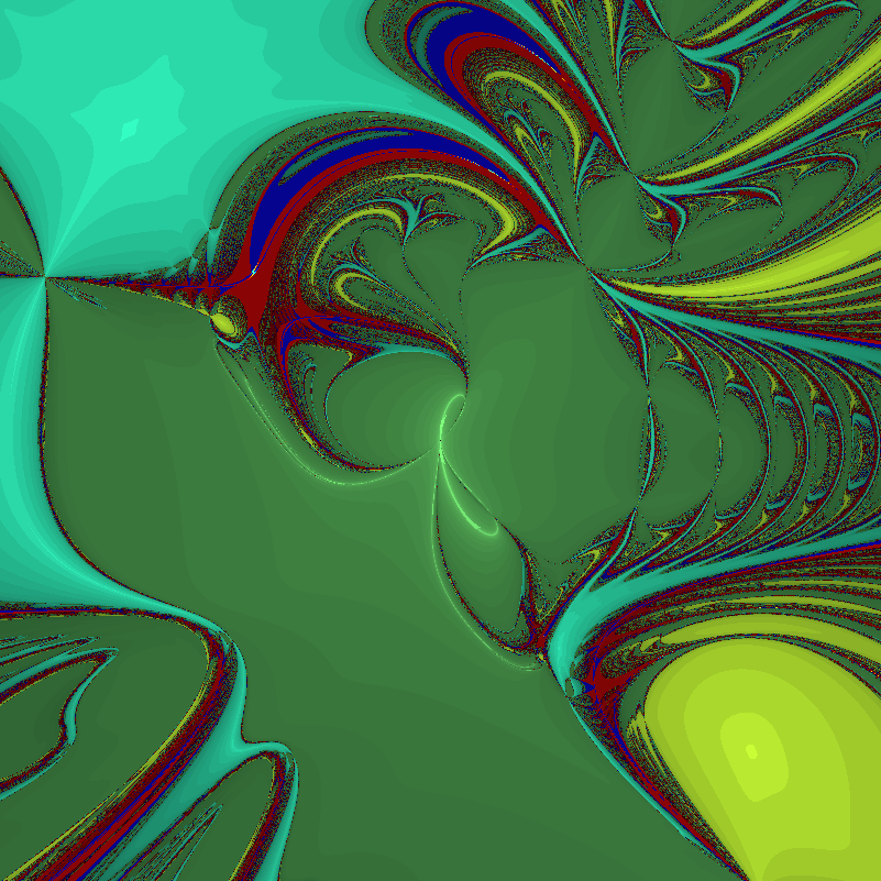
![F=[x^3-3xy^2-1, 3x^2y-y^3]](http://s0.wp.com/latex.php?latex=F%3D%5Bx%5E3-3xy%5E2-1%2C+3x%5E2y-y%5E3%5D&bg=ffffff&fg=000000&s=0 "F=[x^3-3xy^2-1, 3x^2y-y^3]") (which produces the archetypal
(which produces the archetypal =z^3-1") Newton fractal).
Newton fractal).![Newton fractal for F=[x^3-3xy^2-1, 3x^2y-y^3].](http://aleph.se/andart2/wp-content/uploads/2016/12/newtonpert0.png)
![F=[x^3-3xy^2-1 + \epsilon x, 3x^2y-y^3]](http://s0.wp.com/latex.php?latex=F%3D%5Bx%5E3-3xy%5E2-1+%2B+%5Cepsilon+x%2C+3x%5E2y-y%5E3%5D&bg=ffffff&fg=000000&s=0 "F=[x^3-3xy^2-1 + \epsilon x, 3x^2y-y^3]") , then for
, then for  we get: