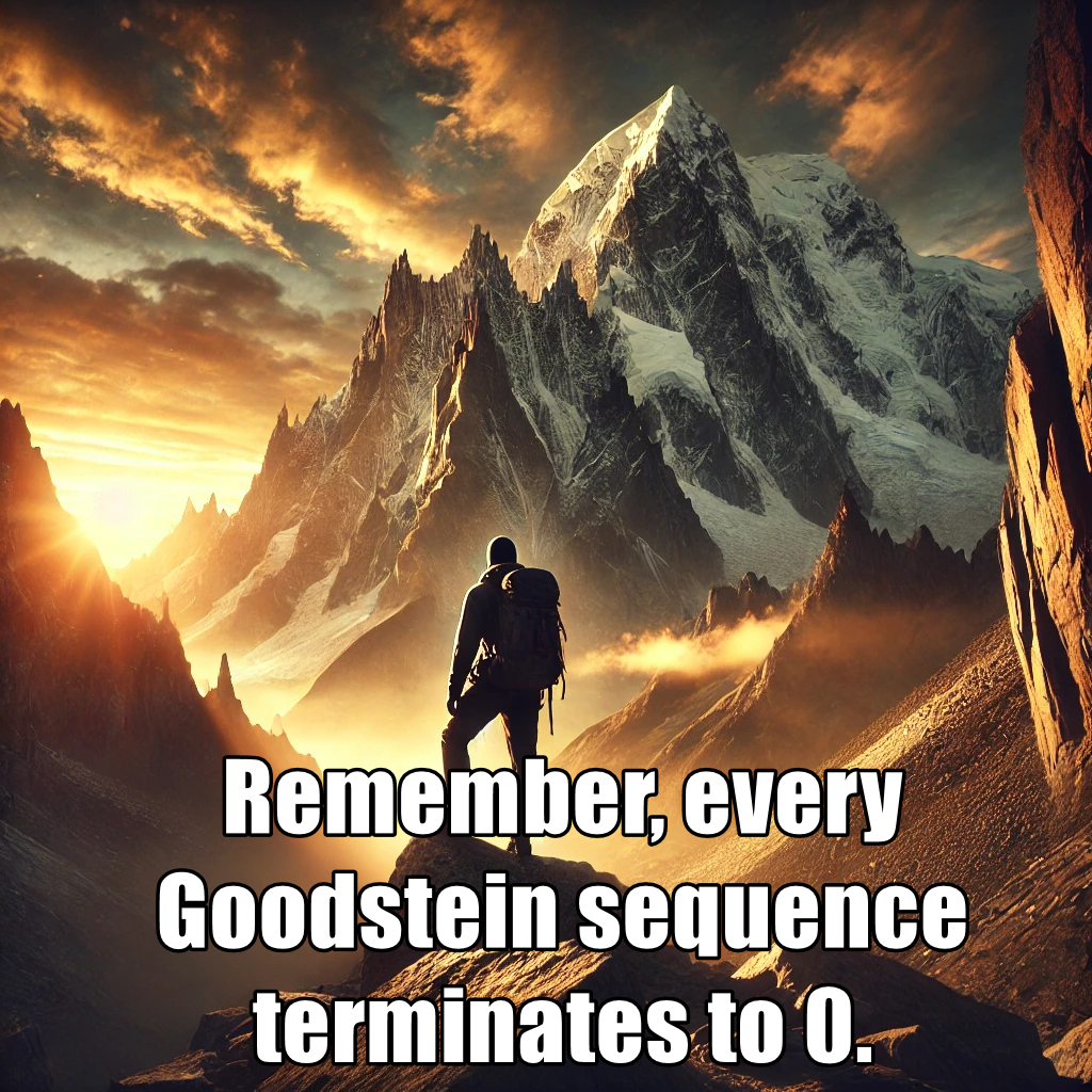
My own exceedingly nerdy motivational poster.
(See Goodstein’s theorem, which is one of the most awesome uses of “let’s complicate things a bit in order to suddenly get a very simple and obvious answer”.)
My own exceedingly nerdy motivational poster.
(See Goodstein’s theorem, which is one of the most awesome uses of “let’s complicate things a bit in order to suddenly get a very simple and obvious answer”.)
What are the weirdest probability distributions I have encountered? Probably the fractal synaptic distribution.
There is no shortage of probability distributions: over any measurable space you can define some function that sums to 1, and you have a probability distribution. Since the underlying space can be integers, rational numbers, real numbers, complex numbers, vectors, tensors, computer programs, or whatever, and the set of functions tends to be big (the power set of the underlying space) there is a lot of stuff out there.
Lists of probability distributions involve a lot of named ones. But for every somewhat recognized distribution there are even more obscure ones.
In normal life I tend to encounter the usual distributions: uniform, Bernouilli, Beta, Gaussians, lognormal, exponential, Weibull (because of survival curves), Erlang (because of sums of exponentials), and a lot of power-laws because I am interested in extreme things.
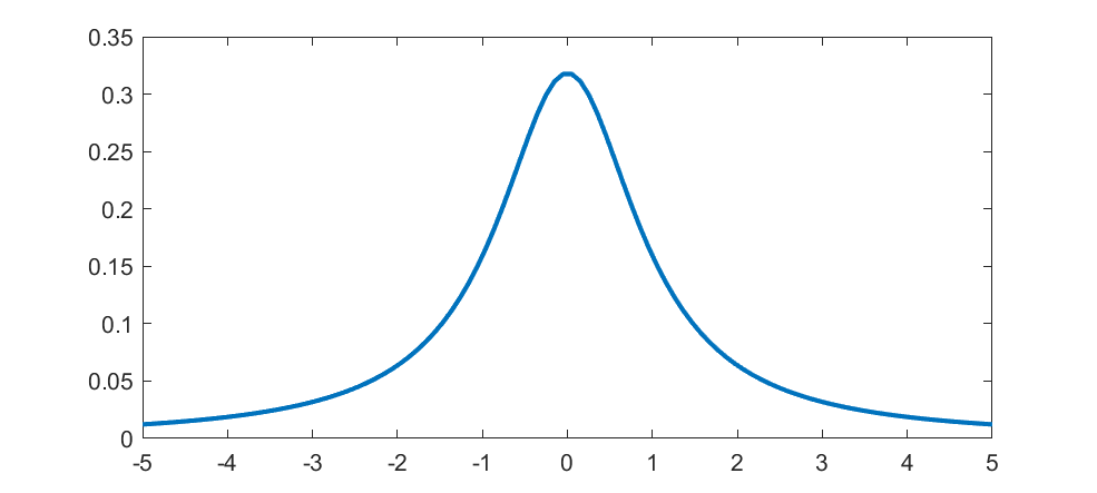 The first “weird” distribution I encountered was the Chauchy distribution. It has a nice algebraic form, a suggestive normalization constant… and no mean, variance or higher order moments. I remember being very surprised as a student when I saw that. It was there on the paper, with a very obvious centre point, yet that centre was not the mean. Like most “pathological examples” it was of course a representative of the majority: having a mean is actually quite “rare”. These days, playing with power-laws, I am used to this and indeed find it practically important. It is no longer weird.
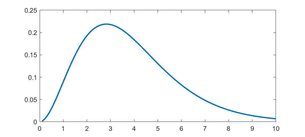 The Planck distribution isn’t too unusual, but has links to many cool special functions and is of course deeply important in physics. It is still surprisingly obscure as a mathematical probability distribution.
The weirdest distribution I have actually used (if only for a forgotten student report) is a fractal.
As a computational neuroscience student I looked into the distribution of synaptic weights in a forgetful attractor memory similar to the Hopfield network. In this case each weight would be updated with a +1 or -1 each time something was learned, added to the previous weight that had decayed somewhat: =k w(t) \pm 1, (0<k<1).")
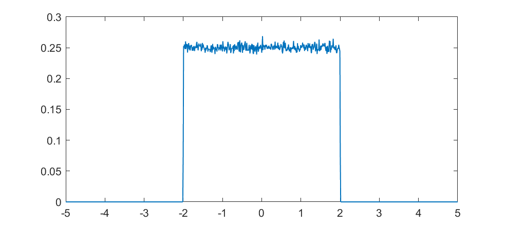
But what about intermediate cases? The update is basically mixing together two copies of the whole distribution. For small k, this produces a distribution across a Cantor set. As k increases the set gets thicker (that is, the fractal dimension increases towards 1), and at k=1/2 you get a uniform distribution. Indeed, it is a strange but true fact that you can not make a uniform distribution over the rational numbers in [0,1] but if we take an infinite sum obviously every single binary sequence will be possible and have equal probability, so it is the real number uniform distribution. Distributions and random numbers on the rationals are funny, since they are both discrete in the sense of being countable, yet so dense that most intuitions from discrete distributions fail and one tends to get fractal/recursive structures.
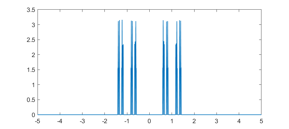
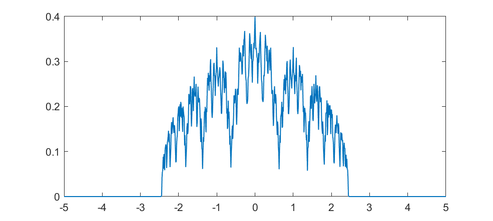
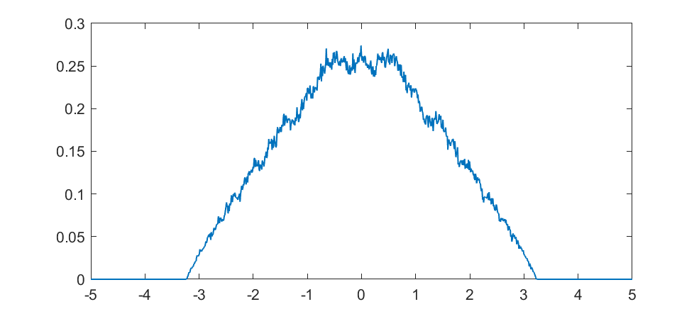
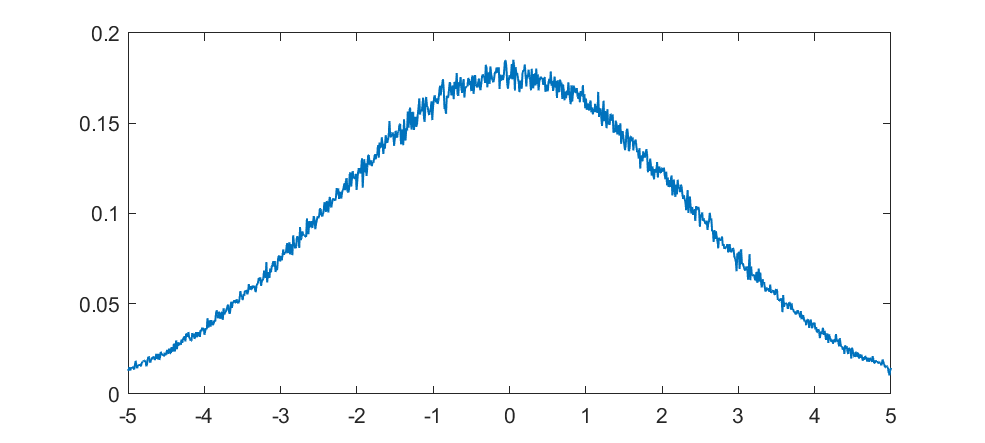
The real fun starts for k>1/2 since now peaks emerge on top of the uniform background. They happen because the two copies of the distribution blended together partially overlap, producing a recursive structure where there is a smaller peak between each pair of big peaks. This gets thicker and thicker, starting to look like a Weierstrass function curve and then eventually a Gaussian.
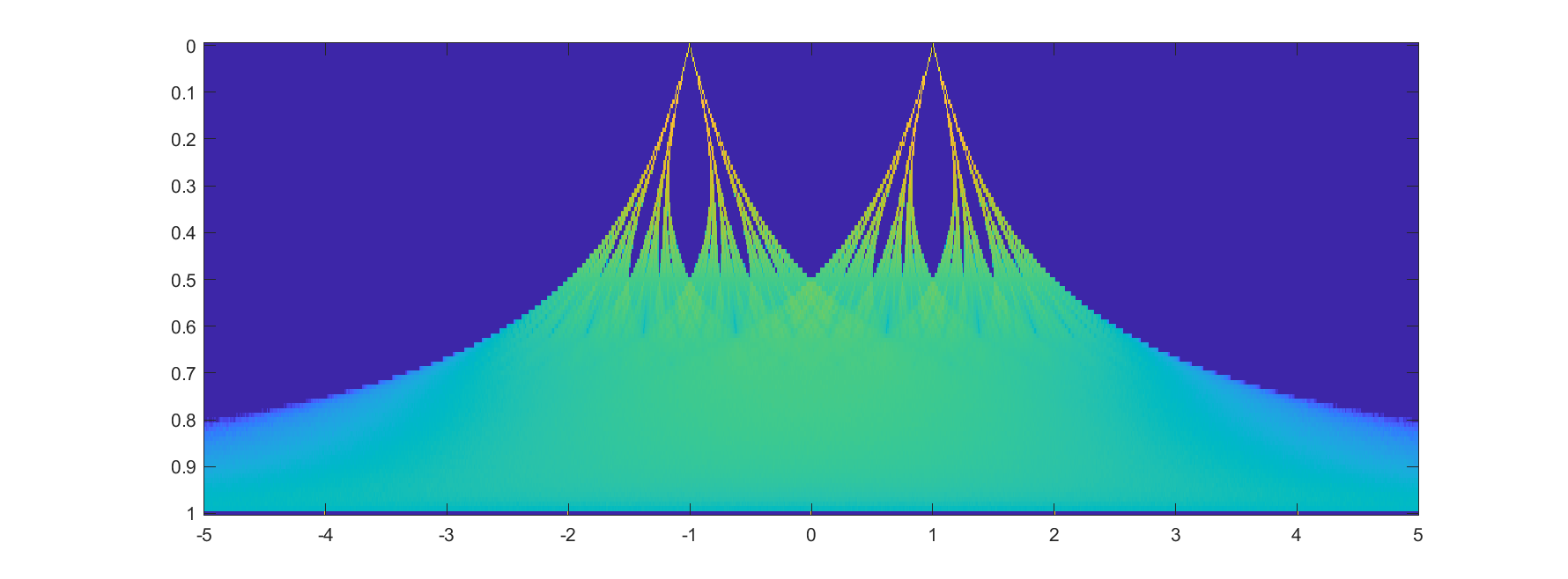
Plotting it in the (x,k) plane shows a neat overall structure, going from the Cantor sets to the fractal distributions towards the Gaussian (and, on the last k=1 row, the discrete Gaussian). The curves defining the edge of the distribution behave as ")
In practice, this distribution is unlikely to matter (real brains are too noisy and synapses do not work like that) but that doesn’t stop it from being neat.
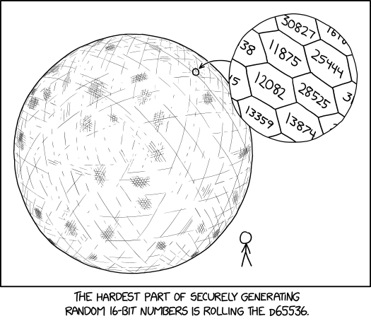
XKCD joked about the problem of secure generation of random 32 bit numbers by rolling a 65536-sided die. Such a die would of course be utterly impractical, but could you actually make a polyhedron that when rolled is a fair dice with 65536 equally likely outcomes?
I immediately tweeted one approach: take a d8 (octahedron), and subdivide each triangle recursively into 4 equal ones, projecting out to a sphere seven times. Then take the dual (vertices to faces, faces to vertices). The subdivision generates 
This is wrong, as Greg Egan himself pointed out. (Note to self: never do math after midnight)
Euler’s formula states that 
F")


This is of course hilariously cursed. It will look almost perfect, but very rarely give numbers outside the expected range.
(What went wrong? My above argument ignored that some vertices – the original polyhedron corners – are different from others.)
Tim Freeman suggested an eminently reasonable approach: start with a tetrahedron, subdivide triangles 7 times with projection outwards, and you end up with a d65536. With triangular sides rather than the mostly hexagonal ones in the cartoon.
But it gets better: when you subdivide a triangle the new vertices are projected out to the surrounding sphere. But that doesn’t mean the four new triangles have the same area. So the areas of the faces are uneven, and we have an unfair die.
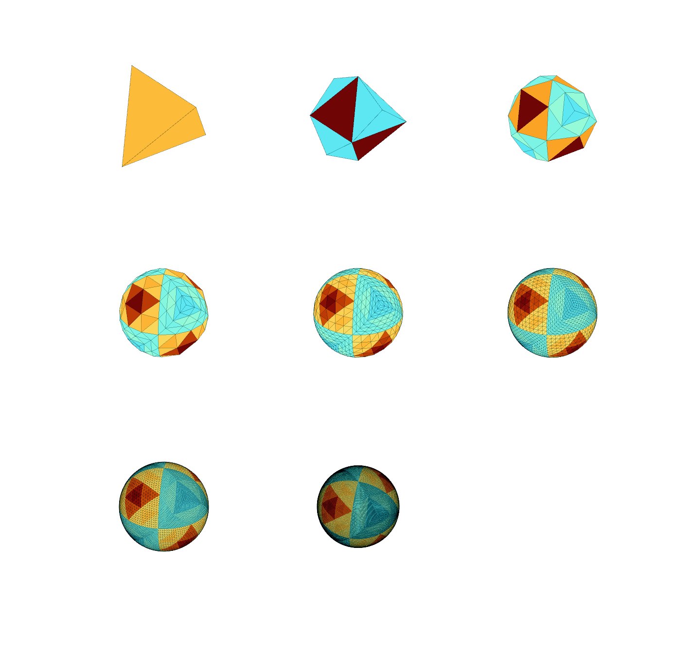 Coloring the sides by relative area shows the fractal pattern of areas.
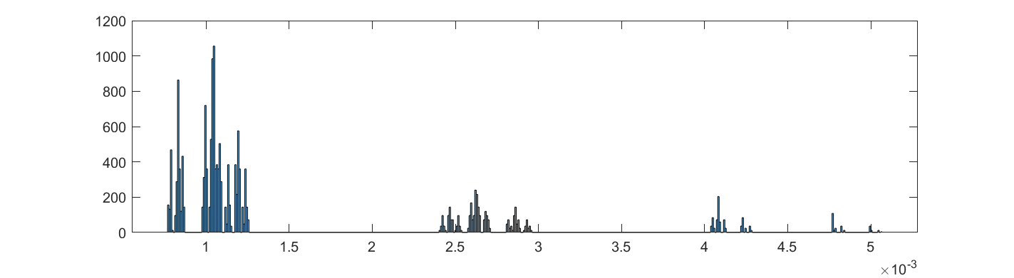 Plotting a histogram of areas show the fractal unevenness. The biggest face has 6.56 times area of the smallest face, so it is not a neglible bias.
One way of solving this is to move the points laterally along the sphere surface to equalize the areas. One can for example use Lloyd’s algorithm. There are many other ways people distribute points evenly on spheres that might be relevant. But subtly unfair giant dice have their own charm.
Note that dice with different face areas can also be fair. Imagine a n-sided prism with length 


Indeed, as discussed in this video, the value of
Dice that are fair by symmetry (and hence under any reasonable throwing dynamics) always have to have an even number of sides and belong to certain symmetry groups (Diaconis & Keller 1989).
A cool way to handle an unfair die is if the assignment of the numbers to the faces are completely scrambled between each roll. It does not matter how uneven the probabilities are, since after being scrambled once the probability of any number being on the most likely face will be the same.
How do you scramble fairly? The obvious approach is a gigantic d(65536!) die, marked with every possible permutation of the faces. This has 
But the previous problems give the nagging question: what if it is unfair?
We can of course scramble the d(65536!) with a d(65536!)! die. If that is fair, then things become fair. But what if we lack such a tremendous die, or there are no big dies that are fair?
Clearly a very unfair d(65536!) can prevent fair d65536-rolling. Imagine that the face with the unit permutation (leave all faces unchanged) has probability 1: the unfairness of the d65536 will remain. If the big die instead has probability close but not exactly 1 for the unit permutation then occasionally it will scramble faces. It could hence make the smaller die fair over long periods (but short-term it would tend to have the same bias towards some faces)… unless the other dominant faces on the d(65536!) were permutations that just moved faces with the same area to each other.
A nearly fair d(65536!) die will on the other hand scramble so that all permutation have some chance of happening, over time allowing the d65536 state to explore the full space of possibility (ergodic dynamics). This seems to be the generic case, with the unfairness-preserving dice as a peculiar special case. In general we should suspect that the typical behavior of mixing occurs: the first few permutations do not change the unfairness much, but after some (usually low) number of permutations the outcomes become very close to the uniform distribution. Hence rolling the d(65536!) die a few times between each roll of the d65536 die and permuting its face numbering accordingly will make it nearly perfectly uniform, assuming the available permutations are irreducible and aperiodic, and that we make enough extra rolls.
How many extra rolls are needed? Suppose all possible permutations are available on the d(65536!) die with nonzero probability. We want to know how many samples from it are needed to make their concatenation nearly uniformly distributed over the 65536! possible ones. If we are lucky the dynamics of the big die creates “rapid mixing dynamics” where this happens after a polynomial times a logarithm steps. Typically the time scales as ")


But, the curse strikes again: we likely need another subdivision scheme to make the d(65536!) die than the d65536 die – this is just a plausibility result, not a proof.
Anyway, XKCD is right that it is hard to get the random bits for cryptography. I suggest flipping coins instead.
A great question from twitter:
Food for thought: There exists some smallest whole number which no human will ever think about.
I wonder how big it is.
— Grant Sanderson (@3blue1brown) January 6, 2020
This is a bit like the “what is the smallest uninteresting number?” paradox, but not paradoxical: we do not have to name it (and hence make it thought about/interesting) to reason about it.
I will first give a somewhat rough probabilistic bound, and then a much easier argument for the scale of this number. TL;DR: the number is likely smaller than 
If we think about 
")
")

If we denote the cumulative distribution function ![P(x)=\Pr[X<x]](http://s0.wp.com/latex.php?latex=P%28x%29%3D%5CPr%5BX%3Cx%5D&bg=ffffff&fg=000000&s=0 "P(x)=\Pr[X<x]")
![F_{(k)}(x) = [P(x)]^{k}](http://s0.wp.com/latex.php?latex=F_%7B%28k%29%7D%28x%29+%3D+%5BP%28x%29%5D%5E%7Bk%7D&bg=ffffff&fg=000000&s=0 "F_{(k)}(x) = [P(x)]^{k}")
}(x^*)=1/2")
What shape does \sim 1/\sqrt{x}")
So if we have 
=\frac{1}{2(k-1)}\frac{1}{\sqrt{x}}")
=(\sqrt{x}-1)/(k-1)")
![F_{(k)}(x)=[(\sqrt{x}-1)/(k-1)]^k](http://s0.wp.com/latex.php?latex=F_%7B%28k%29%7D%28x%29%3D%5B%28%5Csqrt%7Bx%7D-1%29%2F%28k-1%29%5D%5Ek&bg=ffffff&fg=000000&s=0 "F_{(k)}(x)=[(\sqrt{x}-1)/(k-1)]^k")
2^{-1/k}+1)^2 \approx k^2 - 2k \ln(2)")

So, how large is $k$ today? Dorogovtsev et al. had on the order of 

Another approach is to assume each human considers a number about once a minute throughout their lifetime (clearly an overestimate given childhood, sleep, innumeracy etc. but we are mostly interested in orders of magnitude anyway and making an upper bound) which we happily assume to be about a century, giving a personal 


But that assumes “random” numbers, and is a very loose upper bound, merely describing a “typical” small unconsidered number. Were we to systematically think through the numbers from 1 and onward we would have the much lower 
One can refine this a bit: if we have time 


Seth Lloyd estimated that the observable universe cannot have performed more than 


This can be used to consider the future too. Computation of our kind can continue until proton decay in 
But the conclusion is clear: if you write a 173 digit number with no particular pattern of digits (a bit more than two standard lines of typing), it is very likely that this number would never have shown up across the history of the entire universe except for your action. And there is a smaller number that nobody – no human, no alien, no posthuman galaxy brain in the far future – will ever consider.
 Continuing my intermittent Newtonmas fractal tradition (2014, 2016, 2018), today I play around with a very suitable fractal based on gravity.
The problem
On Physics StackExchange NiveaNutella asked a simple yet tricky to answer question:
If we have two unmoving equal point masses in the plane (let’s say at ")
User Kasper showed that one can reframe the problem in terms of elliptic coordinates and show that this implies a straight boundary, while User Lineage showed it more simply using the second constant of motion. I have the feeling that there ought to be an even simpler argument. Still, Kasper’s solution show that the generic trajectory will quasiperiodically fill a region and tend to come arbitrarily close to one of the masses.
The fractal
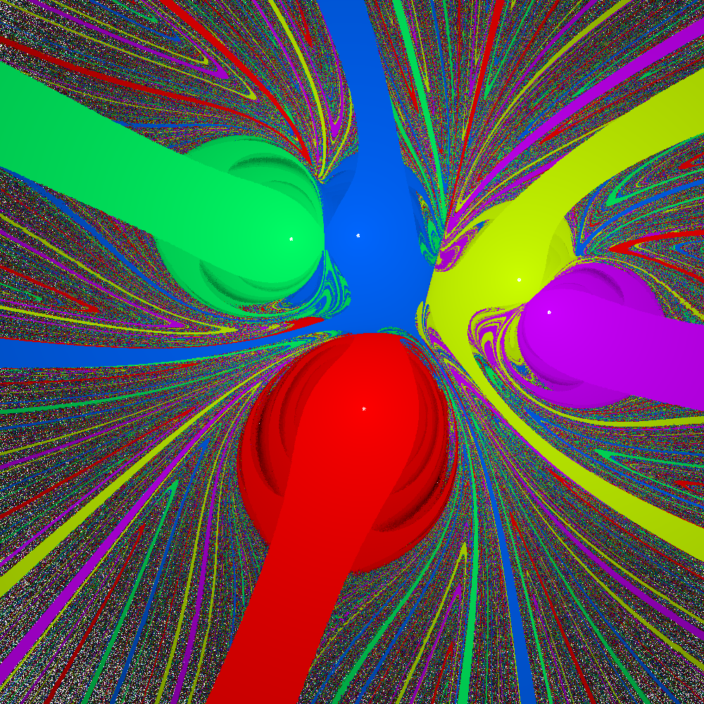
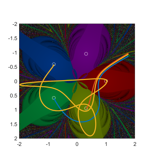
In any case, here is a plot of the basins of attraction shaded by the time until getting within a small radius 
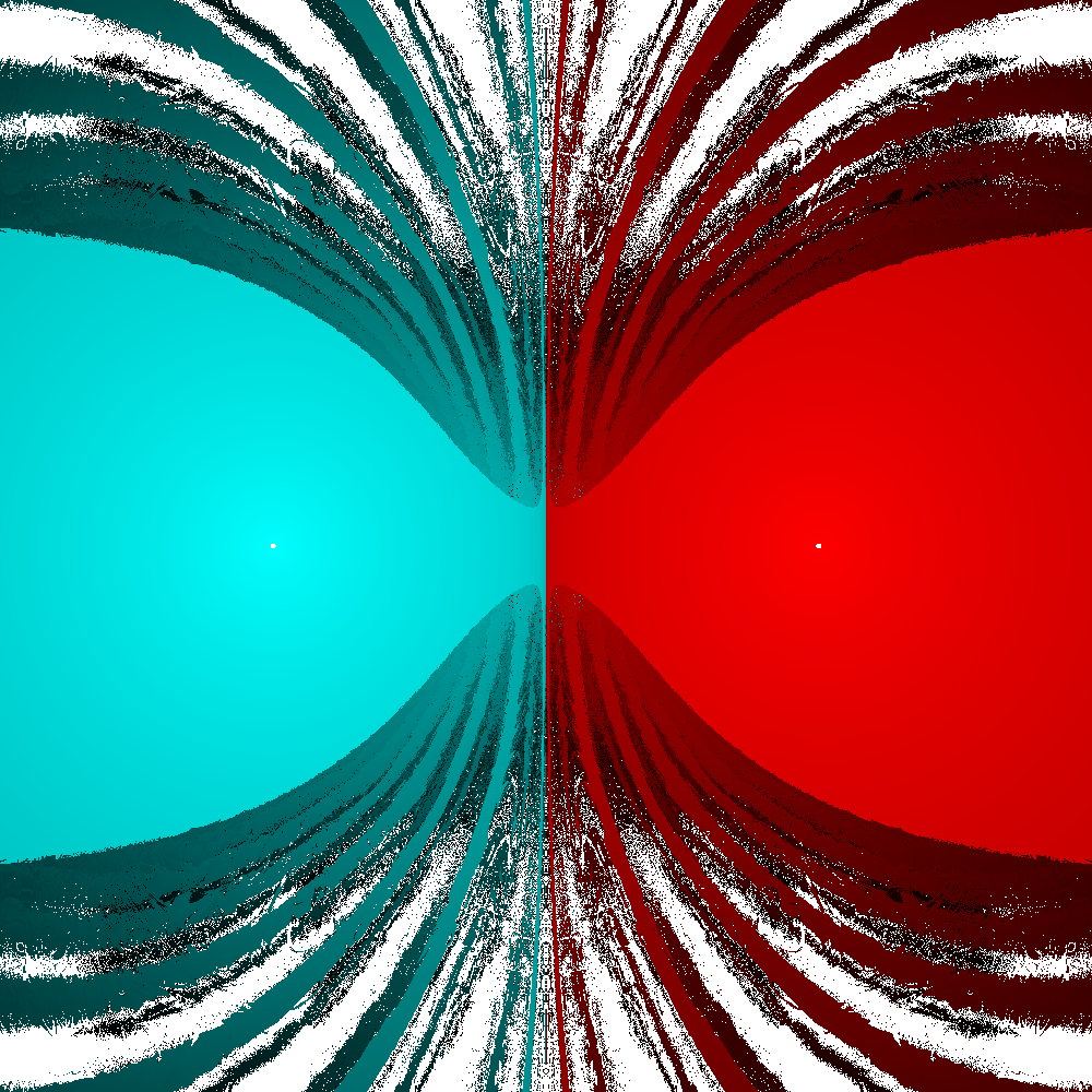
The boundary is a straight line, and surrounding the simple regions where orbits fall nearly straight into the nearest mass are the wilder regions where orbits first rock back and forth across the x-axis before settling into ellipses around the masses.
The case for 5 evenly spaced masses for 

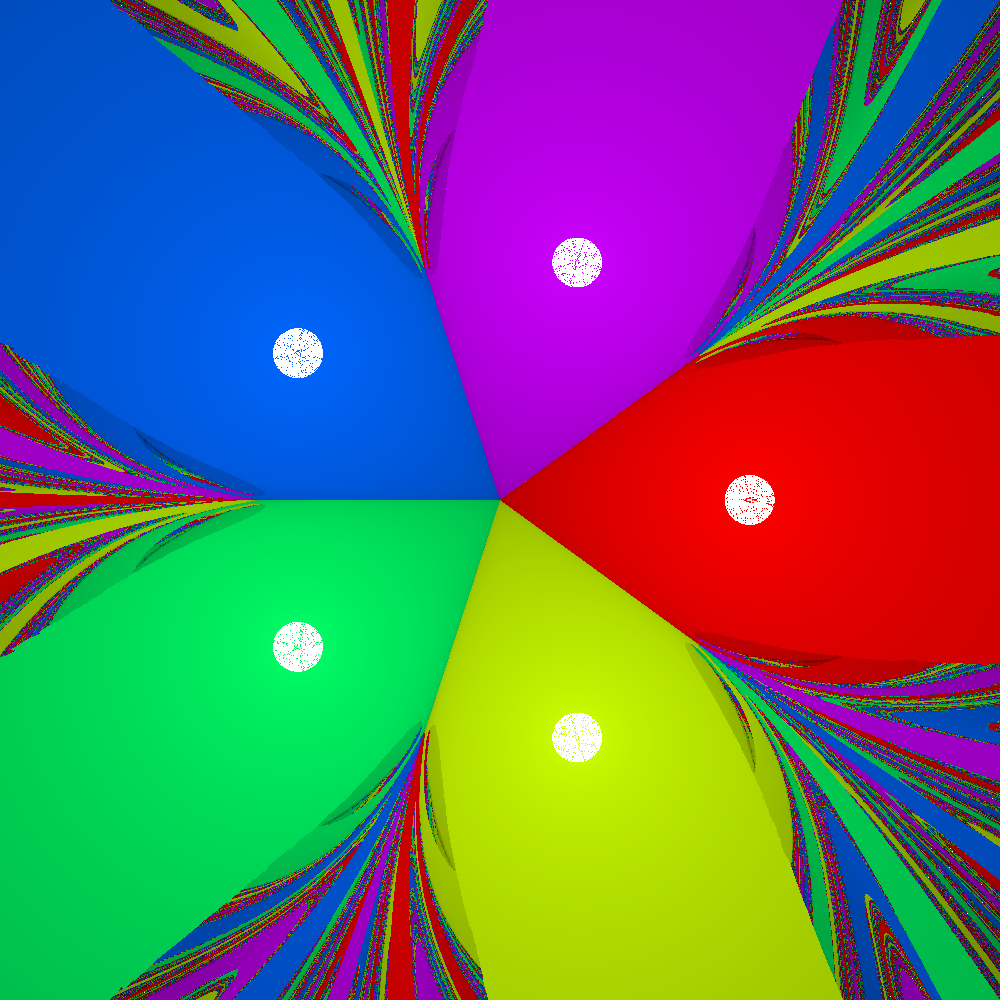

As 
I cannot claim credit for this fractal, as NiveaNutella already plotted it. But it still fascinates me.

Wada basins and mille-feuille collision manifolds
These patterns are somewhat reminiscent of the classic Newton’s root-finding iterative formula fractals: several basins of attraction with a fractal border where pairs of basins encounter interleaved tiny parts of basins not member of the pair.
However, this dynamics is continuous rather than discrete. The plane is a 2D section through a 4D phase space, where starting points at zero velocity accelerate so that they bob up and down/ana and kata along the velocity axes. This also leads to a neat property of the basins of attraction: they are each arc-connected sets, since for any two member points that are the start of trajectories they end up in a small ball around the attractor mass. One can hence construct a map from ![[0,1]](http://s0.wp.com/latex.php?latex=%5B0%2C1%5D&bg=ffffff&fg=000000&s=0 "[0,1]")
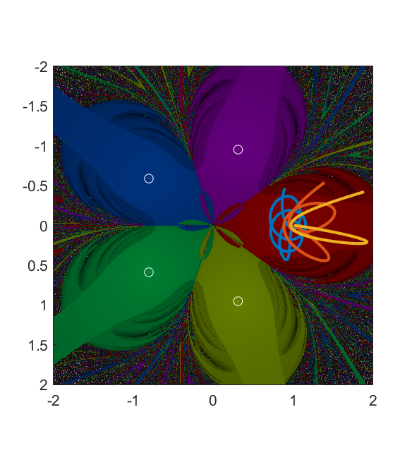
")
Each mass is surrounded by a set of trajectories hitting it exactly, which we can parametrize by the angle they make and the speed they have inwards when they pass some circle around the mass point. They hence form a 3D manifold 
")


The magnetic pendulum
This fractal is similar to one I made back in 1990 inspired by the dynamics of the magnetic decision-making desk toy, a pendulum oscillating above a number of magnets. Eventually it settles over one. The basic dynamics is fairly similar (see Zhampres’ beautiful images or this great treatment). The difference is that the gravity fractal has no dissipation: in principle orbits can continue forever (but I end when they get close to the masses or after a timeout) and in the magnetic fractal the force dependency was bounded, a ")

That simulation was part of my epic third year project in the gymnasium. The topic was “Chaos and self-organisation”, and I spent a lot of time reading the dynamical systems literature, running computer simulations, struggling with WordPerfect’s equation editor and producing a manuscript of about 150 pages that required careful photocopying by hand to get the pasted diagrams on separate pieces of paper to show up right. My teacher eventually sat down with me and went through my introduction and had me explain Poincaré sections. Then he promptly passed me. That was likely for the best for both of us.
Appendix: Matlab code
showPlot=0; % plot individual trajectories
randMass = 0; % place masses randomly rather than in circle

RTRAP=0.0001; % size of trap region
tmax=60; % max timesteps to run
S=1000; % resolution

x=linspace(-2,2,S);
y=linspace(-2,2,S);
[X,Y]=meshgrid(x,y);

N=5;
theta=(0:(N-1))*pi*2/N;
PX=cos(theta); PY=sin(theta);
if (randMass==1)
s = rng(3);
PX=randn(N,1); PY=randn(N,1);
end

clf

hit=X*0;
hitN = X*0; % attractor basin
hitT = X*0; % time until hit
closest = X*0+100;
closestN=closest; % closest mass to trajectory

tic; % measure time
for a=1:size(X,1)
disp(a)
for b=1:size(X,2)
[t,u,te,ye,ie]=ode45(@(t,y) forceLaw(t,y,N,PX,PY), [0 tmax], [X(a,b) 0 Y(a,b) 0],odeset('Events',@(t,y) finishFun(t,y,N,PX,PY,RTRAP^2)));

if (showPlot==1)
plot(u(:,1),u(:,3),'-b')
hold on
end

if (~isempty(te))
hit(a,b)=1;
hitT(a,b)=te;

mind2=100^2;
for k=1:N
dx=ye(1)-PX(k);
dy=ye(3)-PY(k);
d2=(dx.^2+dy.^2);
if (d2<mind2) mind2=d2; hitN(a,b)=k; end
end

end
for k=1:N
dx=u(:,1)-PX(k);
dy=u(:,3)-PY(k);
d2=min(dx.^2+dy.^2);
closest(a,b)=min(closest(a,b),sqrt(d2));

if (closest(a,b)==sqrt(d2)) closestN(a,b)=k; end
end
end

if (showPlot==1)
drawnow
pause
end
end
elapsedTime = toc

if (showPlot==0)
% Make colorful plot
co=hsv(N);
mag=sqrt(hitT);
mag=1-(mag-min(mag(:)))/(max(mag(:))-min(mag(:)));
im=zeros(S,S,3);
im(:,:,1)=interp1(1:N,co(:,1),closestN).*mag;
im(:,:,2)=interp1(1:N,co(:,2),closestN).*mag;
im(:,:,3)=interp1(1:N,co(:,3),closestN).*mag;
image(im)
end

% Gravity
function dudt = forceLaw(t,u,N,PX,PY)
%dudt = zeros(4,1);
dudt=u;
dudt(1) = u(2);
dudt(2) = 0;
dudt(3) = u(4);
dudt(4) = 0;

dx=u(1)-PX;
dy=u(3)-PY;
d=(dx.^2+dy.^2).^-1.5;
dudt(2)=dudt(2)-sum(dx.*d);
dudt(4)=dudt(4)-sum(dy.*d);

% for k=1:N
% dx=u(1)-PX(k);
% dy=u(3)-PY(k);
% d=(dx.^2+dy.^2).^-1.5;
% dudt(2)=dudt(2)-dx.*d;
% dudt(4)=dudt(4)-dy.*d;
% end
end

% Are we close enough to one of the masses?
function [value,isterminal,direction] =finishFun(t,u,N,PX,PY,r2)
value=1000;
for k=1:N
dx=u(1)-PX(k);
dy=u(3)-PY(k);
d2=(dx.^2+dy.^2);
value=min(value, d2-r2);
end
isterminal=1;
direction=0;
end
It is Newtonmass, and that means doing some fun math. I try to invent a new fractal or something similar every year: this is the result for 2018.
The Newton fractal is an old classic. Newton’s method for root finding iterates an initial guess 
/f'(z_{n})")
\neq 0")
The Newton-Gauss method is a method for minimizing the total squared residuals =\sum_{i=1}^m r_i^2(\beta)")

=f(x_i;\beta)-y_i")
")
^{-1}J^t r(\beta)")


So we can make fractals by trying to fit (say) a function consisting of the sum of two Gaussians with different means (but fixed variances) to a random set of points. So we can set ![f(x;\beta_1,\beta_2)=(1/\sqrt{2\pi})[e^{-(x-\beta_1)^2/2}+(1/4)e^{-(x-\beta_1)^2/8}]](http://s0.wp.com/latex.php?latex=f%28x%3B%5Cbeta_1%2C%5Cbeta_2%29%3D%281%2F%5Csqrt%7B2%5Cpi%7D%29%5Be%5E%7B-%28x-%5Cbeta_1%29%5E2%2F2%7D%2B%281%2F4%29e%5E%7B-%28x-%5Cbeta_1%29%5E2%2F8%7D%5D&bg=ffffff&fg=000000&s=0 "f(x;\beta_1,\beta_2)=(1/\sqrt{2\pi})[e^{-(x-\beta_1)^2/2}+(1/4)e^{-(x-\beta_1)^2/8}]")
")
It is a bit modernistic-looking. As I argued in 2016, this is because the generic local Jacobian of the dynamics doesn’t have much rotation.
As more and more points are added the attractor landscape becomes simpler, since it is hard for the Gaussians to “stick” to some particular clump of points and the gradients become steeper.
This fractal can obviously be generalized to more dimensions by using more parameters for the Gaussians, or more Gaussians etc.
The fractality is guaranteed by the generic property of systems with several attractors that points at the border of two basins of attraction will tend to find their ways to other attractors than the two equally balanced neighbors. Hence a cut transversally across the border will find a Cantor-set of true basin boundary points (corresponding to points that eventually get mapped to a singular Jacobian in the iteration formula, like the boundary of the Newton fractal is marked by points mapped to =0")
Merry Newtonmass!
I recently came across this nice animated gif of a fractal based on a Steiner chain, due to Eric Martin Willén. I immediately wanted to replicate it.
First, how do you make a Steiner chain? It is easy using inversion geometry. Just decide on the number of circles tangent to the inner circle (
)/(1+\sin(\pi/n))")
/2")
/2")
![]()
![]()
Since the original concentric chain obviously can be rotated continuously without losing touch with the inner and outer circle, this also generates a continuous family of circles after the inversion. This is why Steiner’s porism is true: if you can make the initial chain, you get an infinite number of other chains with the same number of circles.
The fractal works by putting copies of the whole set of circles in the chain into each circle, recursively. I remap the circles so that the outer circle becomes the unit circle, and then it is easy to see that for a given small circle with (complex) centre 
=(w+z)r")
Done.
Except… it feels a bit dry.
Ever since I first encountered iterated function systems in the 1980s I have felt they tend towards a geometric aesthetics that is not me, ferns notwithstanding. A lot has to do with the linearity of the transformations. One can of course add rotations, which cheers up the fractal a bit.
But still, I love the nonlinearity and harmony of conformal mappings.
Enter the circle inversion fractals. They are the sets of the plane that map to themselves when being inverted in any and all of a set of generating circles (or, equivalently, the limit set of points under these inversions). As a rule of thumb, when the circles do not touch the fractal will be Cantor/Fatou-style fractal dust. When the circles are tangent the fractal will pass through the point of tangency. If three circles are tangent the fractal will contain a circle passing through these points. Since Steiner chains have lots of tangencies, we should get a lot of delicious fractals by using them as generators.
I use nearly the same code I used for the elliptic inversion fractals, mostly because I like the colours. The “real” fractal is hidden inside the nested circles, composed of an infinite Apollonian gasket of circles.
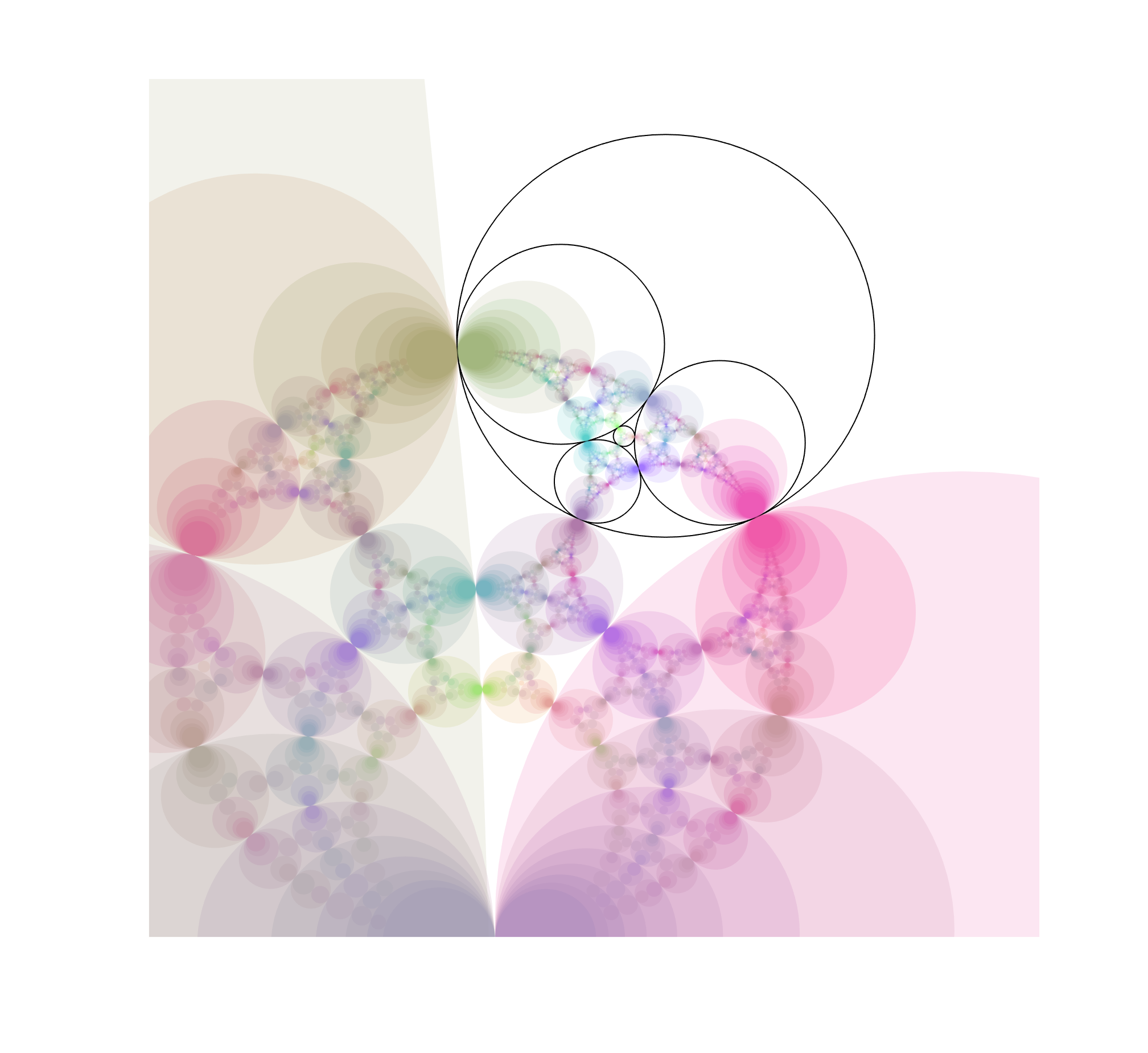

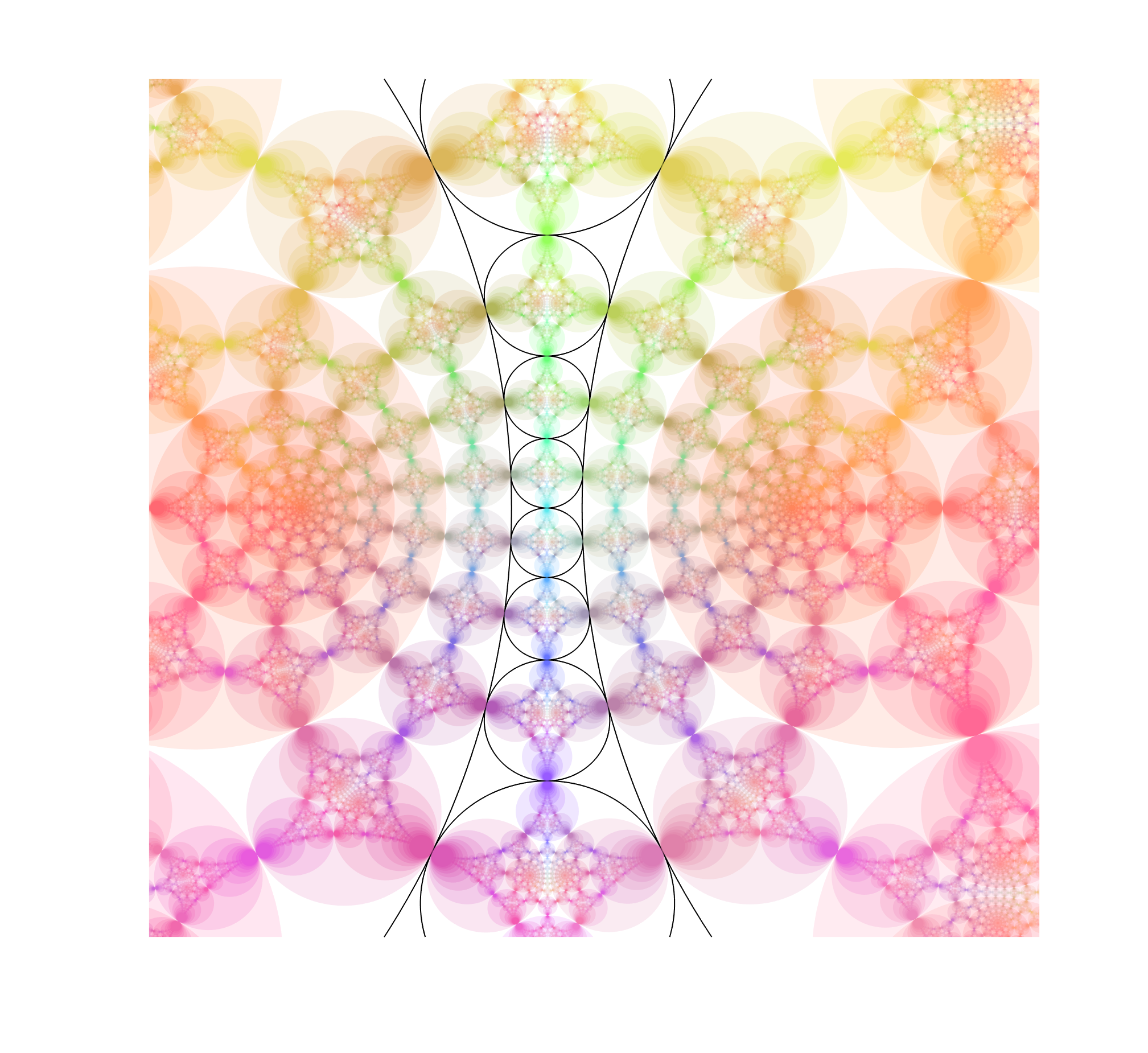
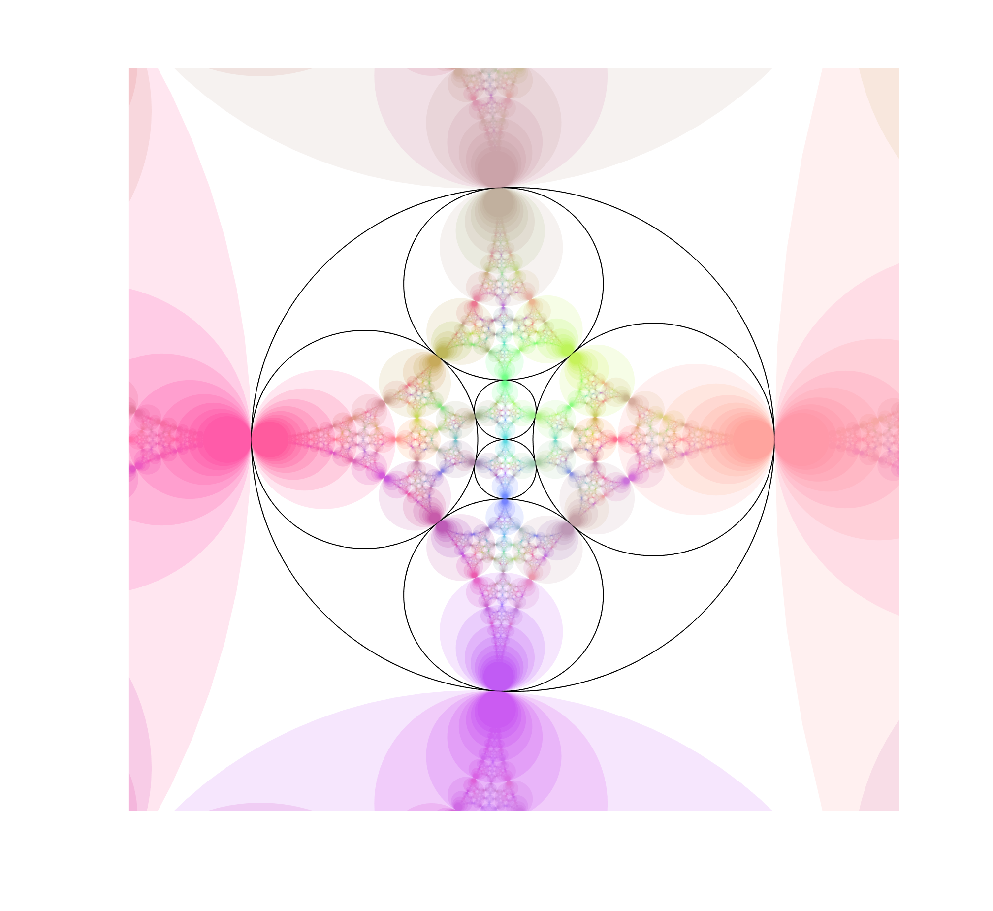

Note how the fractal extends outside the generators, forming a web of circles. Convergence is slow near tangent points, making it “fuzzy”. While it is easy to see the circles that belong to the invariant set that are empty, there are also circles going through the foci inside the coloured disks, touching the more obvious circles near those fuzzy tangent points. There is a lot going on here.
But we can complicate things by allowing the chain to slide and see how the fractal changes.
This is pretty neat.
Here is a minimal surface based on the Weierstrass-Enneper representation =1, g(z)=\tanh^2(z)")
![\Re([-\tanh(z)(\mathrm{sech}^2(z)-4)/6,i(6z+\tanh(z)(\mathrm{sech}^2(z)-4))/6,z-\tanh(z)])](http://s0.wp.com/latex.php?latex=%5CRe%28%5B-%5Ctanh%28z%29%28%5Cmathrm%7Bsech%7D%5E2%28z%29-4%29%2F6%2Ci%286z%2B%5Ctanh%28z%29%28%5Cmathrm%7Bsech%7D%5E2%28z%29-4%29%29%2F6%2Cz-%5Ctanh%28z%29%5D%29&bg=ffffff&fg=000000&s=0 "\Re([-\tanh(z)(\mathrm{sech}^2(z)-4)/6,i(6z+\tanh(z)(\mathrm{sech}^2(z)-4))/6,z-\tanh(z)])")
It is based on my old tanh surface, but has a wilder style. It gets helped by the fact that my triangulation in the picture is pretty jagged. On one hand it has two flat ends, but also a infinite number of catenoid openings (only two shown here).
I call it Håkan’s surface, since I came up with it on my dear husband’s birthday. Happy birthday, Håkan!
I recently returned to toying around with circle and sphere inversion fractals, that is, fractal sets that are invariant under inversion in a given set of circles or spheres.
That got me thinking: can you invert points in other things than circles? Of course you can! José L. Ramírez has written a nice overview of inversion in ellipses. Basically a point 


In Cartesian coordinates, for an ellipse centered on the origin and with semimajor and minor axes 
")
")


Many of the properties remain the same. Lines passing through the centre of the ellipse are unchanged. Other lines get mapped to ellipses; if they intersect the inversion ellipse the new ellipse also intersect it at those points. Hence tangent lines are mapped to tangent ellipses. Ellipses with parallel axes and equal eccentricities map onto other ellipses (or lines if they intersect the centre of the inversion ellipse). Other conics get turned into cubics; for example a hyperbola gets mapped to a lemniscate. (See also this paper for more examples).
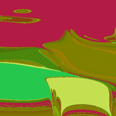
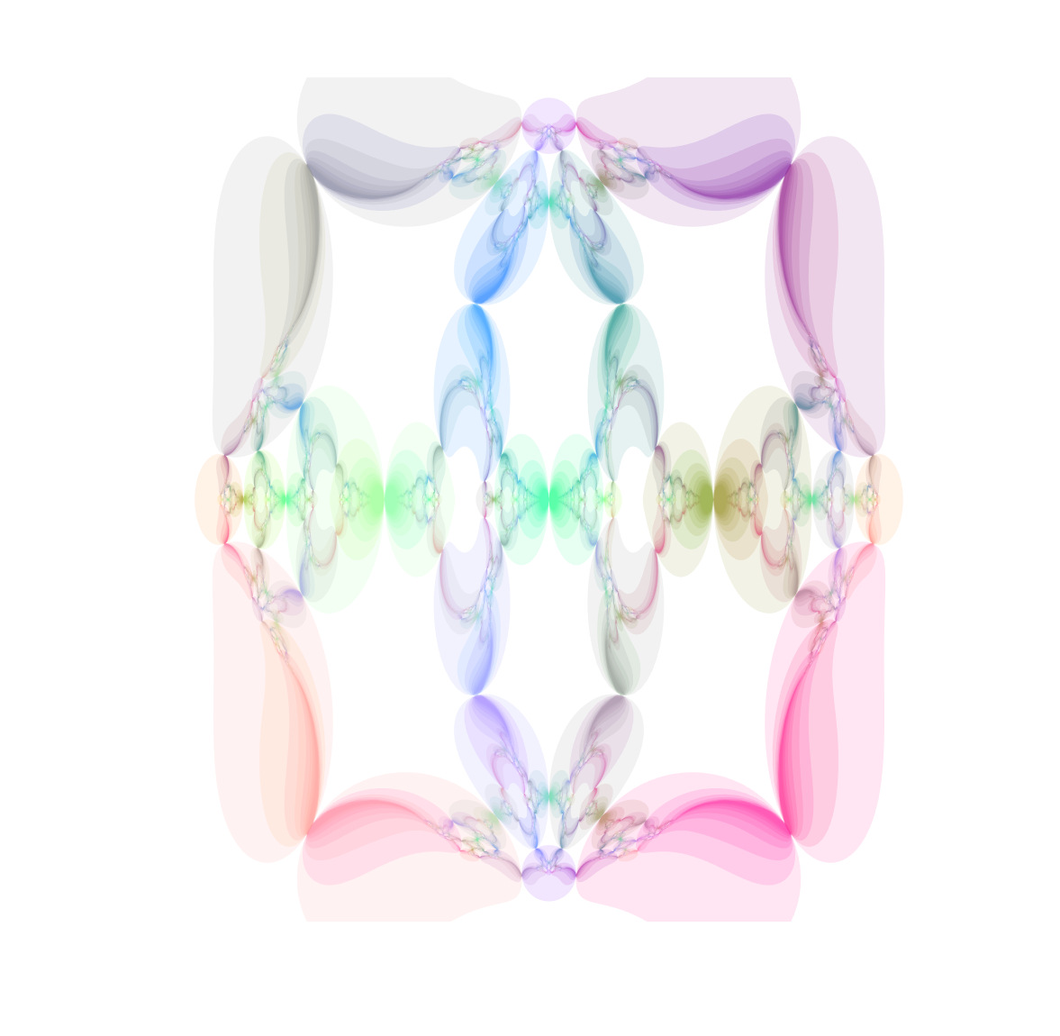
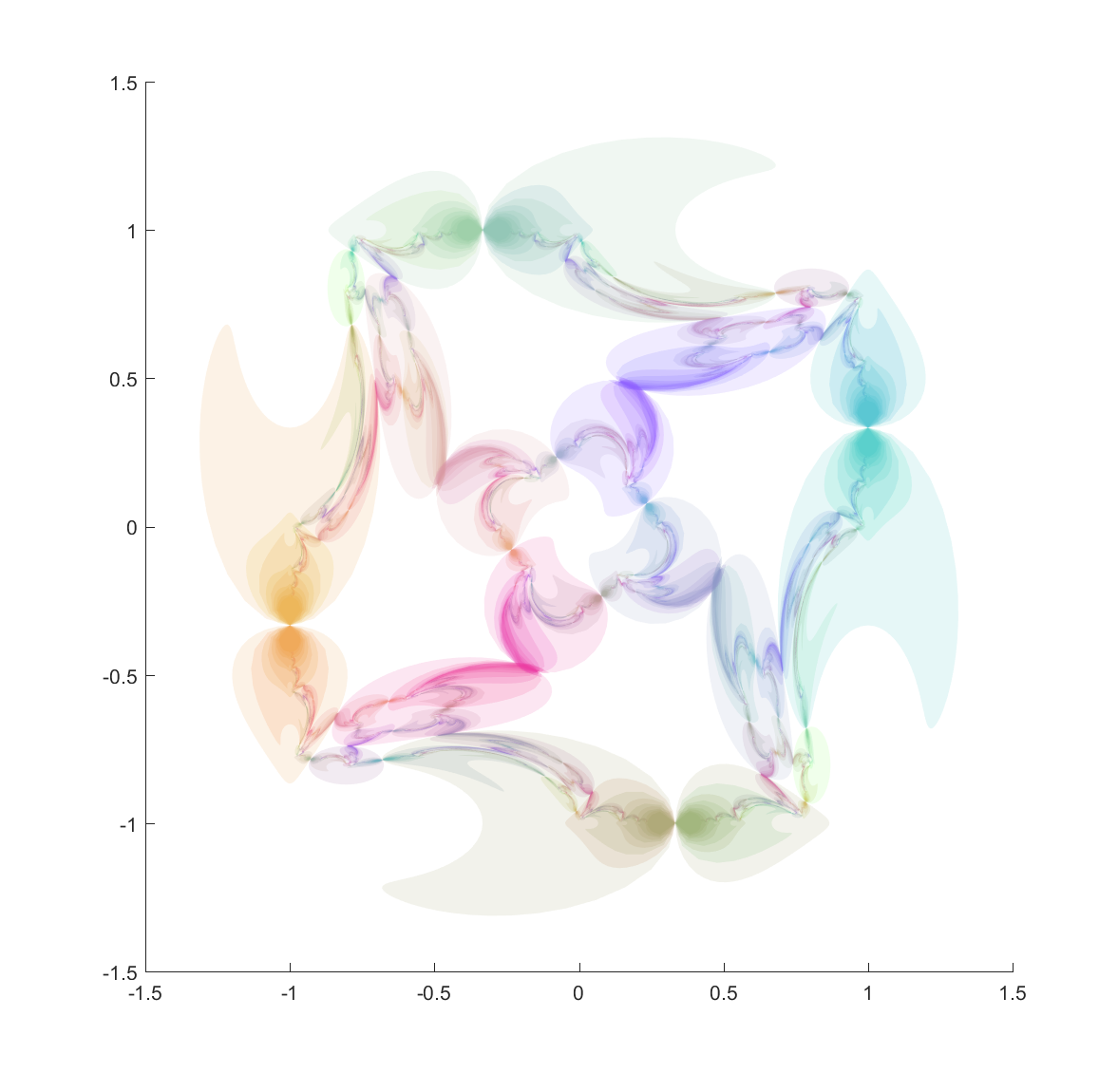
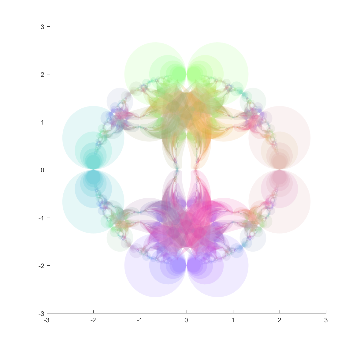
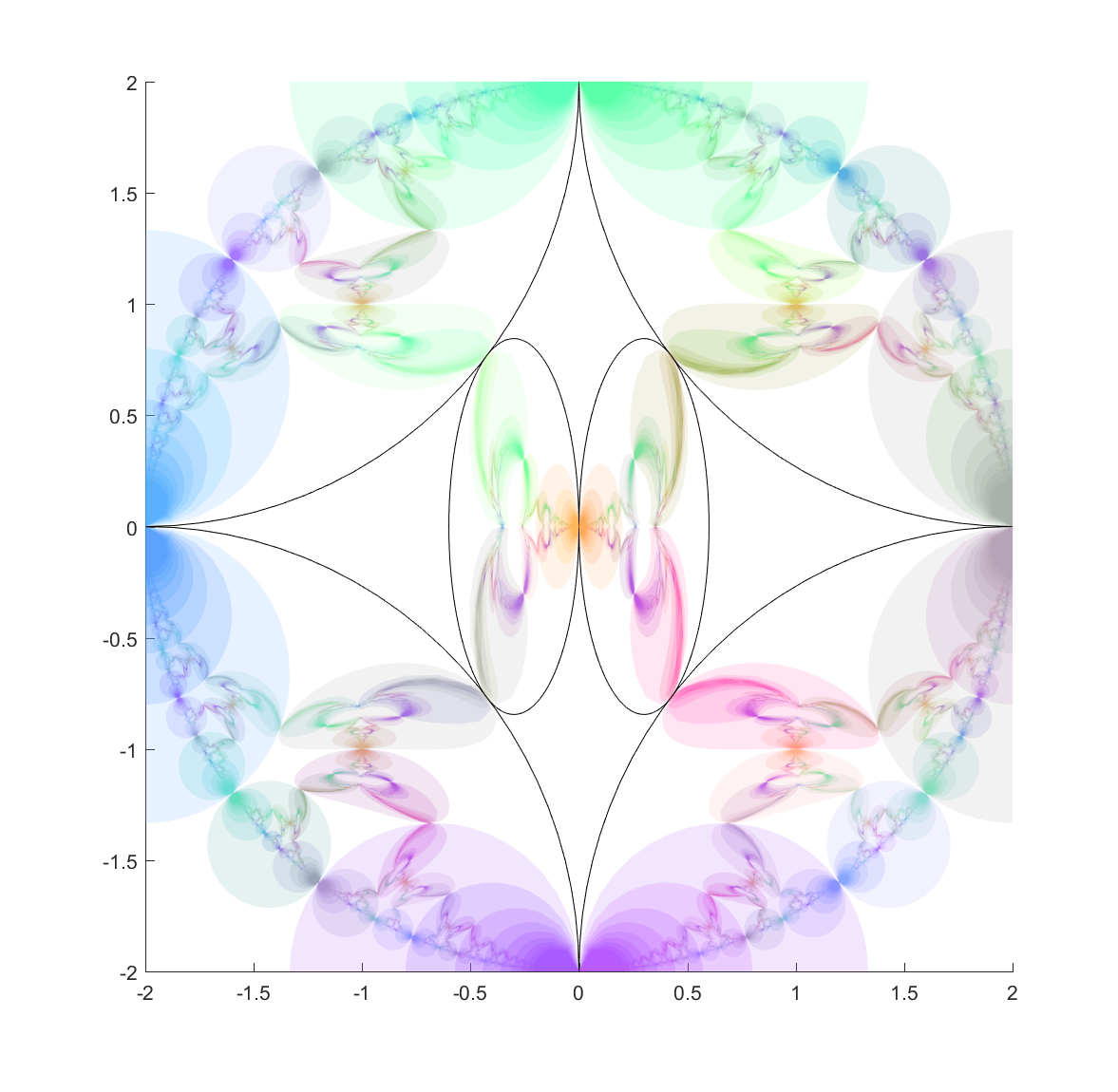
Now, from a fractal standpoint this means that if you have a set of ellipses that are tangent you should expect a fractal passing through their points of tangency. Basically all of the standard circle inversion fractals hence have elliptic counterparts. Here is the result for a ring of 4 or 6 mutually tangent ellipses:
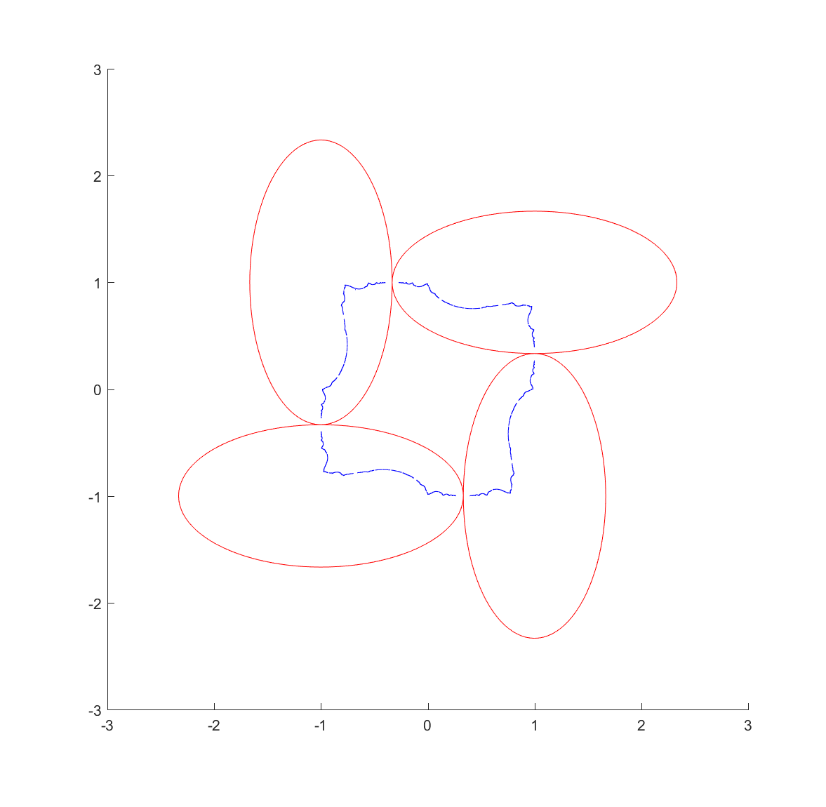
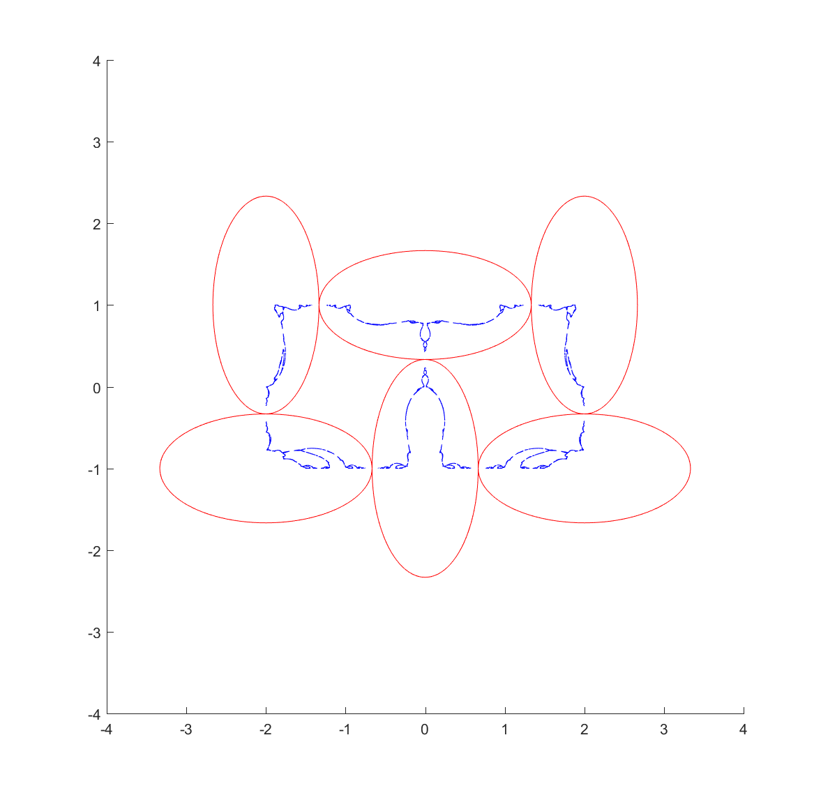
These pictures were generated by taking points in the plane and inverting them with randomly selected ellipses; as the process continues they get attracted to the invariant set (this is basically a standard iterated function system). It also has the known problem of finding the points at the tangencies, since the iteration has to loop consistently between inverting in the two ellipses to get there, but it is likely that a third will be selected at some point.
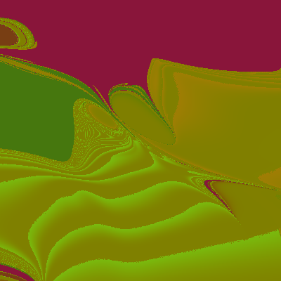
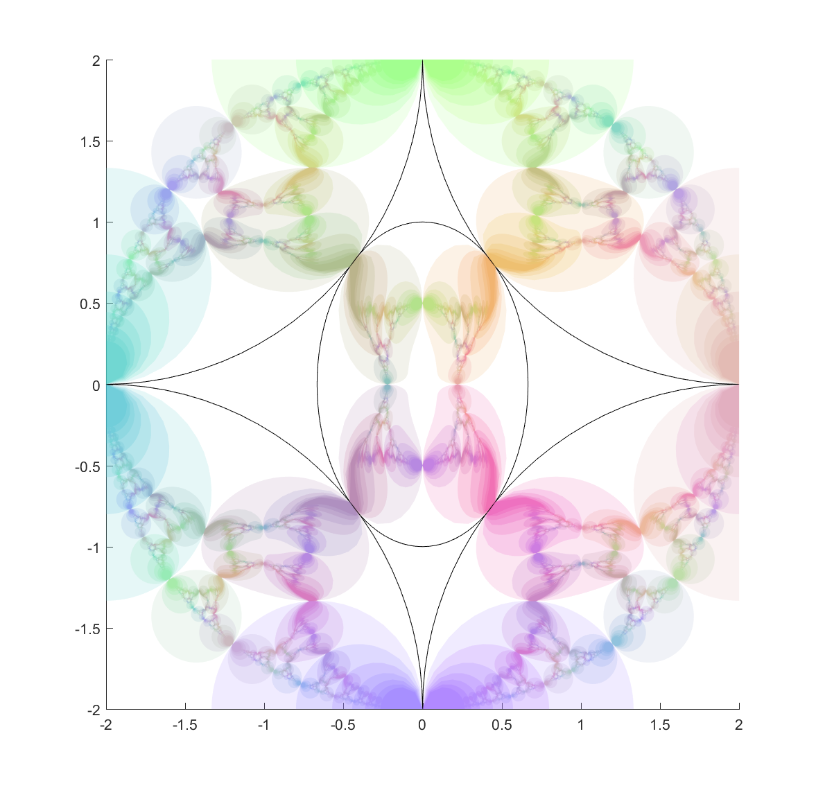
One approach is to deliberately recurse downward to find the points using a depth first search. We can take look at where each ellipse is mapped by each of the inversions, and since the fractal is inside each of the mapped ellipses we can then continue mapping the chain of mapped ellipses, getting nice bounds on where it is going (as long as everything is shrinking: this is guaranteed as long as it is mappings from the outside to the inside of the generating ellipses, but if they were to overlap things can explode). Doing this for just one step reveals one reason for the quirky shapes above: some of the ellipses get mapped into crescents or pears, adding a lot of bends:
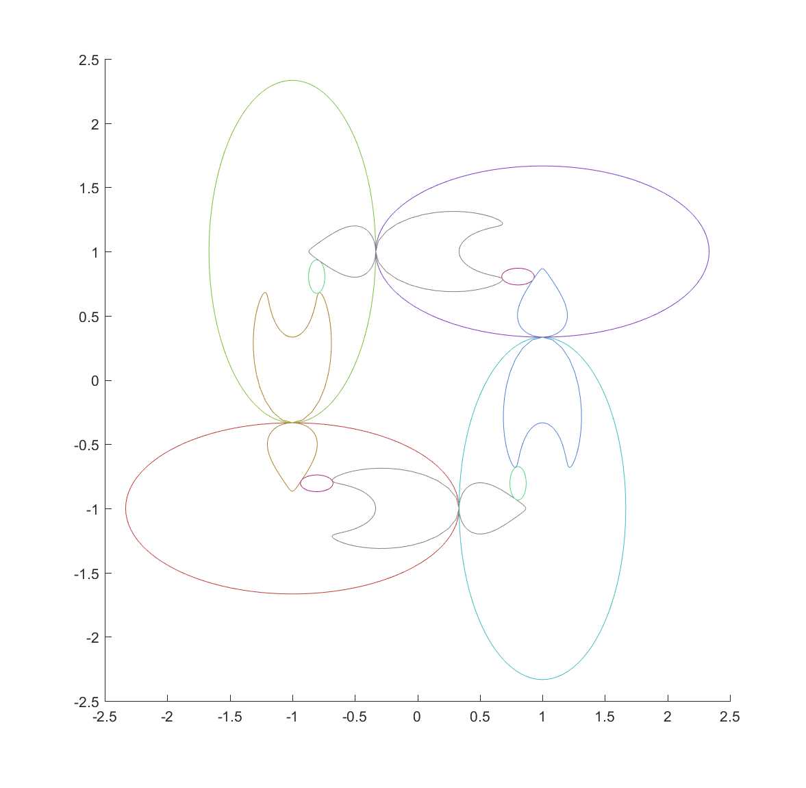
Now, continuing this process makes a nested structure where the invariant set is hidden inside all the other mapped ellipses.
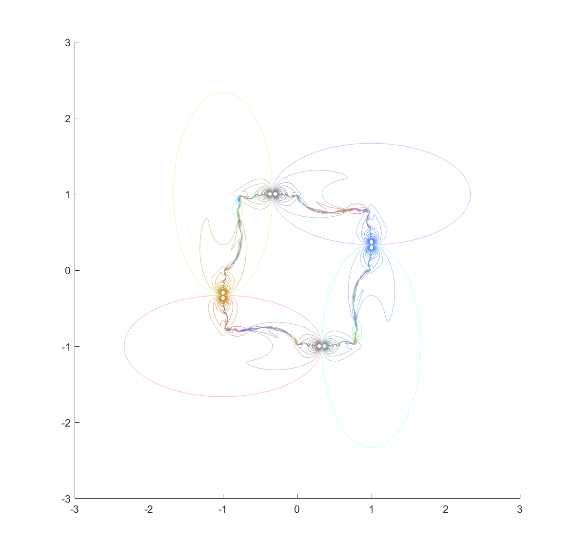
It is still hard to reach the tangent points, but at least now they are easier to detect. They are also numerically tough: most points on the ellipse circumferences are mapped away from them towards the interior of the generating ellipse. Still, if we view the mapped ellipses as uncertainties and shade them in we can get a very pleasing map of the invariant set:
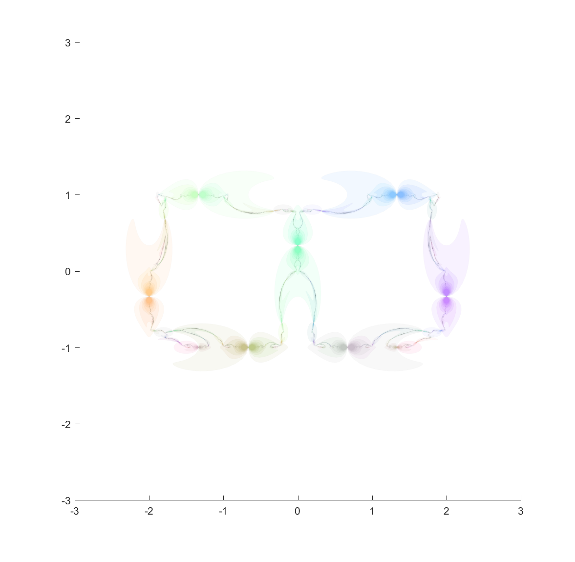
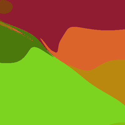
Here are a few other nice fractals based on these ideas:
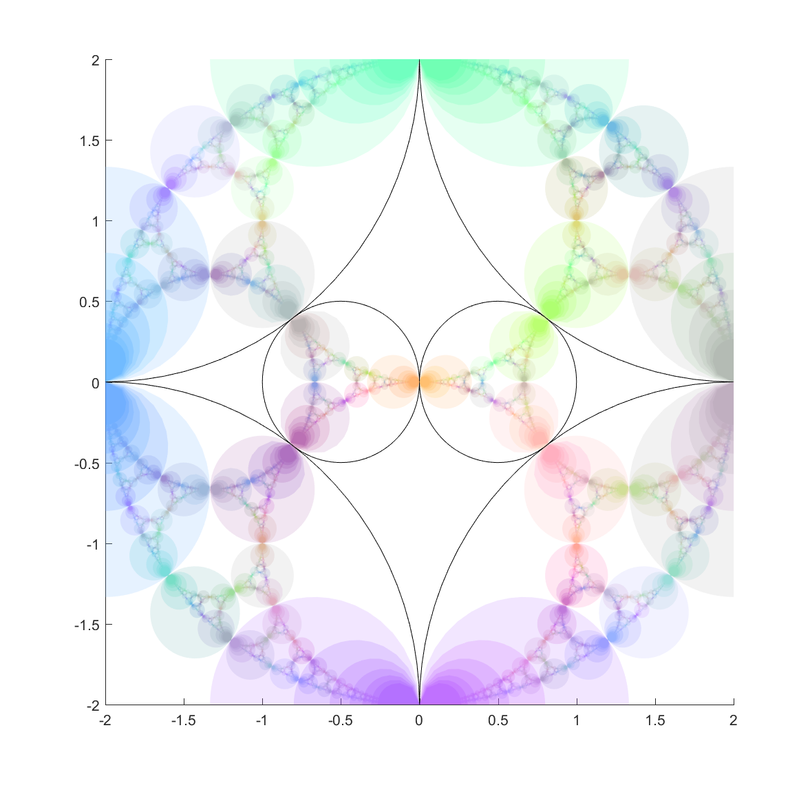
Using a mix of circles and ellipses produces a nice mix of the regularity of the circle-based Apollonian gaskets and the swooshy, Hénon fractal shape the ellipses induce.
% center=[-1 -1 2 1; -1 1 1 2; 1 -1 1 2; 1 1 2 1];
% center(:,3:4)=center(:,3:4)*(2/3);
%
%center=[-1 -1 2 1; -1 1 1 2; 1 -1 1 2; 1 1 2 1; 3 1 1 2; 3 -1 2 1];
%center(:,3:4)=center(:,3:4)*(2/3);
%center(:,1)=center(:,1)-1;
%
% center=[-1 -1 2 1; -1 1 1 2; 1 -1 1 2; 1 1 2 1];
% center(:,3:4)=center(:,3:4)*(2/3);
% center=[center; 0 0 .51 .51];
%
% egg
% center=[0 0 0.6666 1; 2 2 2 2; -2 2 2 2; -2 -2 2 2; 2 -2 2 2];
%
% double
%r=0.5;
%center=[-r 0 r r; r 0 r r; 2 2 2 2; -2 2 2 2; -2 -2 2 2; 2 -2 2 2];
%
% Double egg
center=[0.3 0 0.3 0.845; -0.3 0 0.3 0.845; 2 2 2 2; -2 2 2 2; -2 -2 2 2; 2 -2 2 2];
%
M=size(center,1); % number of ellipses
N=100; % points on fill curves
X=randn(N+1,2);
clf
hold on
tt=2*pi*(0:N)/N;
alpha 0.2
for i=1:M
    X(:,1)=center(i,1)+center(i,3)*cos(tt);
    X(:,2)=center(i,2)+center(i,4)*sin(tt);
    plot(X(:,1),X(:,2),'k');
    for j=1:M
        if (i~=j)
            recurseDown(X,[i j],10,center)
            drawnow
       end
    end
end
function recurseDown(X,ellword,maxlevel,center)
i=ellword(end); % invert in latest ellipse
%
% Perform inversion
C=center(i,1:2);
A2=center(i,3).^2;
B2=center(i,4).^2;
Y(:,1)=X(:,1)-C(:,1);
Y(:,2)=X(:,2)-C(:,2);
X(:,1)=C(:,1)+A2.*B2.*Y(:,1)./(B2.*Y(:,1).^2+A2.*Y(:,2).^2);
X(:,2)=C(:,2)+A2.*B2.*Y(:,2)./(B2.*Y(:,1).^2+A2.*Y(:,2).^2);
%
if (norm(max(X)-min(X))<0.005) return; end
%
co=hsv(size(center,1));
coco=mean([1 1 1; 1 1 1; co(ellword,:)]);
%
%    plot(X(:,1),X(:,2),'Color',coco)
fill(X(:,1),X(:,2),coco,'FaceAlpha',.2,'EdgeAlpha',0)
%
if (length(ellword)<maxlevel)
    for j=1:size(center,1)
        if (j~=i)
            recurseDown(X,[ellword j],maxlevel,center)
        end
    end
end
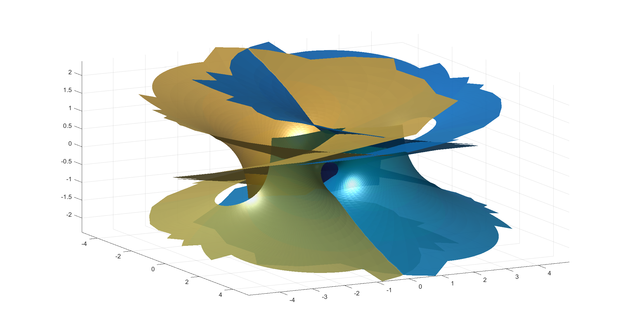
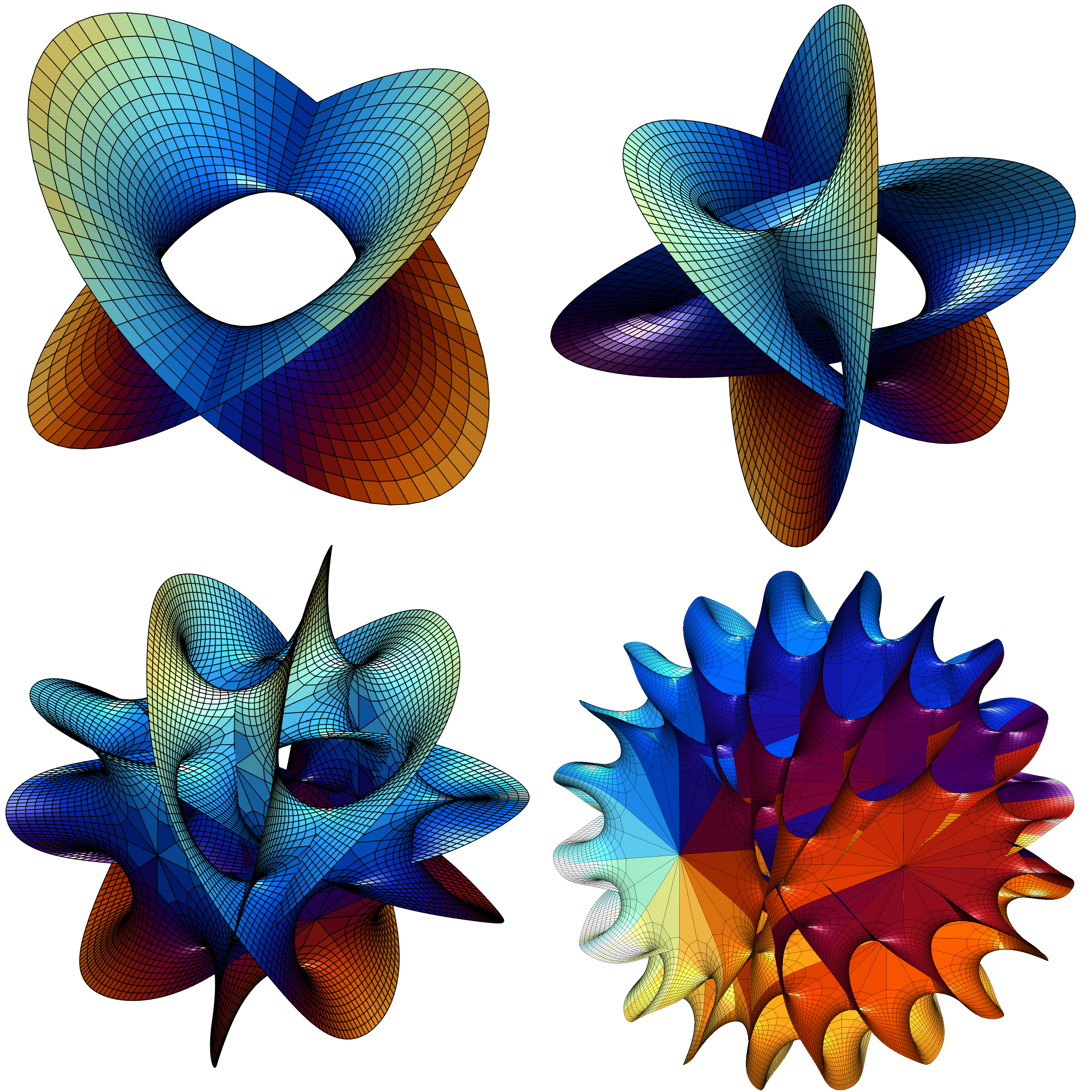
I have a glass cube on my office windowsill containing a slice of a Calabi-Yau manifold, one of Bathsheba Grossman’s wonderful creations. It is an intricate, self-intersecting surface with lots of unexpected symmetries. A visiting friend got me into trying to make my own version of the surface.
First, what is the equation for it? Grossman-Hanson’s explanation is somewhat involved, but basically what we are seeing is a 2D slice through a 6-dimensional manifold in a projective space expressed as the 4D manifold 
where the k’s run through ")

where 
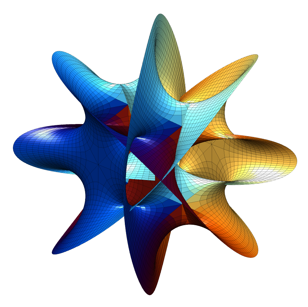
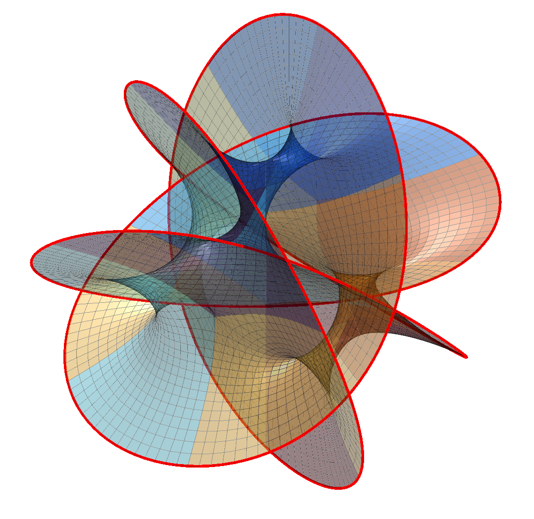
The result is pretty nifty. It is tricky to see how it hangs together in 2D; rotating it in 3D helps a bit. It is composed of 16 identical patches:
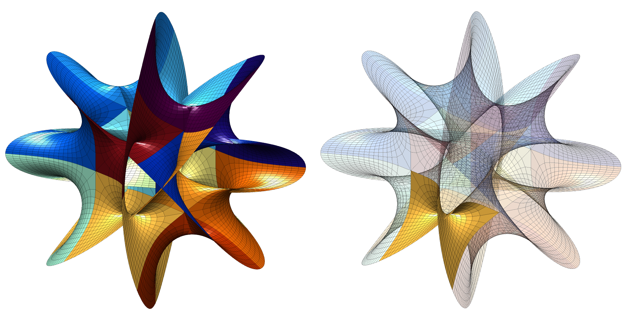
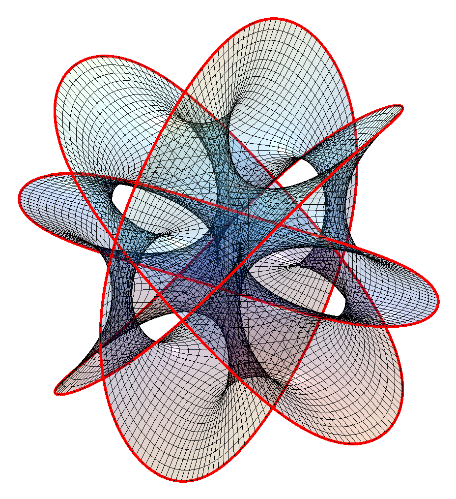
The boundary of the patches meet other patches except along two open borders (corresponding to large or small values of 
A surface bounded by a knot or a link is called a Seifert surface. While these surfaces look a lot like minimal surfaces they are not exactly minimal when I estimate the mean curvature (it should be exactly zero); while this could be because of lack of numerical precision I think it is real: while minimal surfaces are Ricci-flat, the converse is not necessarily true.
Changing N produces other surfaces. N=2 is basically a catenoid (tilted and self-intersecting). As N increases it becomes more like a barrel or a pufferfish, with one direction dominated by circular saddle regions, one showing a meshwork of spaces reminiscent of spacefilling minimal surfaces, and one a lot of overlapping “barbs”.
Note that just like for minimal surfaces one can multiply 

Hanson also notes that by changing the formula to 
%% Initialization

edge=0; % Mark edge?

coloring=1; % Patch coloring type

n=4;

s=0.1; % Gridsize

alp=1; ca=cos(alp); sa=sin(alp); % Projection

[theta,xi]=meshgrid(-1.5:s:1.5,1*(pi/2)*(0:1:16)/16);

z=theta+xi*i;

% Color scheme

tt=2*pi*(1:200)'/200; co=.5+.5*[cos(tt) cos(tt+1) cos(tt+2)];

colormap(co)

%% Plot

clf

hold on

for k1=0:(n-1)

for k2=0:(n-1)

z1=exp(k1*2*pi*i/n)*cosh(z).^(2/n);

z2=exp(k2*2*pi*i/n)*(1/i)*sinh(z).^(2/n);

X=real(z1);

Y=real(z2);

Z=ca*imag(z1)+sa*imag(z2);

if (coloring==0)

surf(X,Y,Z);

else

switch (coloring)

case 1

C=z1*0+(k1+k2*n); % Color by patch

case 2

C=abs(z1);

case 3

C=theta;

case 4

C=xi;

case 5

C=angle(z1);

case 6

C=z1*0+1;

end

h=surf(X,Y,Z,C);

set(h,'EdgeAlpha',0.4)

end

if (edge>0)

plot3(X(:,end),Y(:,end),Z(:,end),'r','LineWidth',2)

plot3(X(:,1),Y(:,1),Z(:,1),'r','LineWidth',2)

end

end

end

view([2 3 1])

camlight

h=camlight('left');

set(h,'Color',[1 1 1]*.5)

axis equal

axis vis3d

axis off
=e^{2\pi i k_1 / n}\cosh(\theta+\xi i)^{2/n}")
=e^{2 \pi i k_2 / n}\sinh(\theta+\xi i)^{2/n}/i")
,\Re(z_2),\cos(\alpha)\Im(z_1)+\sin(\alpha)\Im(z_2))")
=e^{2\pi i k_1 / n_1}\cosh(\theta+\xi i)^{2/n_1}")
=e^{2 \pi i k_2 / n_2}\sinh(\theta+\xi i)^{2/n_2}/i")