Apropos Newton’s method in the complex plane, what happens when the degree of the polynomial goes to infinity?
Towards infinity
Obviously there will be more zeros, so there will be more attractors and we should expect the boundaries of the basins of attraction to become messier. But it is not entirely clear where the action will be, so it would be useful to compress the entire complex plane into a convenient square.
How do you depict the entire complex plane? While I have always liked the Riemann sphere here I tried mapping to . The origin is unchanged, and infinity becomes the edges of the square . This is not a conformal map, so things will get squished near the edges.
For color, I used to map complex coordinates to RGB. This makes the color depend on the distance to 1, -1 and i, making infinity white and zero some drab color (the -1 terms at the end determines the overall color range).
Here is the animated result:
What is going on? As I scale up the size of the leading term from zero, the root created by adding that term moves in from infinity towards the center, making the new basin of attraction grow. This behavior has been described in this post on dancing zeros. The zeros also tend to cluster towards the unit circle, crowding together and distributing themselves evenly. That distribution is the reason for the the colorful “flowers” that surround white spots (poles of the Newton formula, corresponding to zeros of the derivative of the polynomial). The central blob is just the attractor of the most “solid” zero, corresponding to the linear and constant terms of the polynomial.
The jostling is amusing: it looks like the roots do repel each other. This is presumably because close roots require a sharp turn of the function, but the “turning radius” is set by the coefficients that tend to be of order unity. Getting degenerate roots requires coefficients to be in a set of measure zero, so it is rare. Near-degenerate roots exist in a positive measure set surrounding that set, but it is still “small” compared to the general case.
At infinity
So what happens if we let the degree go to infinity? As I previously mentioned, the generic behaviour of where is independent random numbers is a lacunary function. So we should not expect anything outside the unit circle. Inside the circle there will be poles, so there will be copies of the undefined outside region (because of Great Picard’s Theorem (meromorphic version)). Since the function is analytic these copies will be conformal mappings of the exterior and hence roughly circular. There will also be zeros, and these will have their own basins of attraction. A few of the central ones dominate, but there is an infinite number of attractors as we approach the circular border which is crammed with poles and zeros.
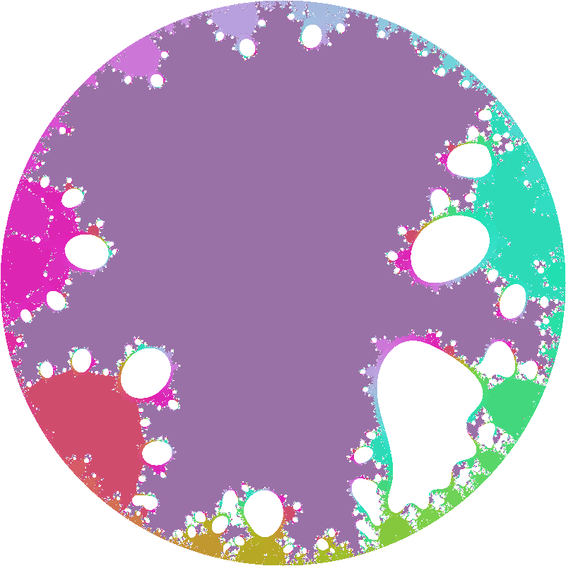
Since we now know we will only deal with the unit disk, we can avoid transforming the entire plane and enjoy the results:
Attractors for random 10,000-degree polynomial.Attractors for random 10,000-degree polynomial.
What happens here is that the white regions represents places where points get mapped onto the undefined outside, while the colored fractal regions are the attraction basins for the zeros. And between them there is a truly wild boundary. In the vanilla fractal every point on the boundary is a meeting point of the three basins, a tri-point. Here there is an infinite number of attractors: the boundary consists of points where an infinite number of different attractors meet.
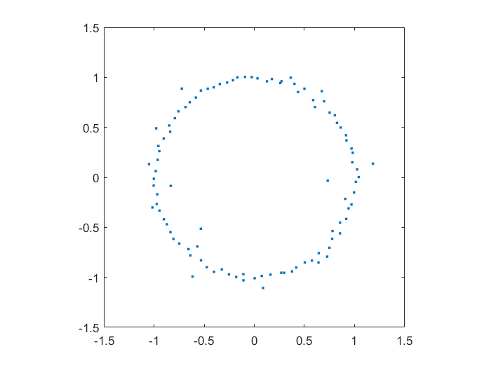
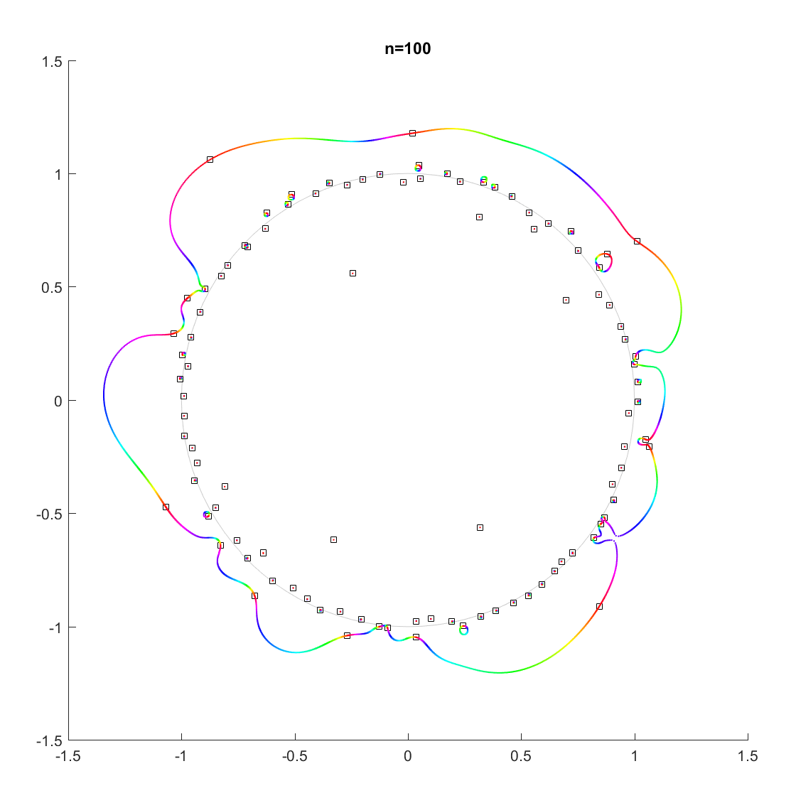
Playing with Matlab, I plotted the location of the zeros of a polynomial with normally distributed coefficients in the complex plane. It was nearly a circle:
Zeros of a 100-degree polynomial with normally distributed random coefficients.
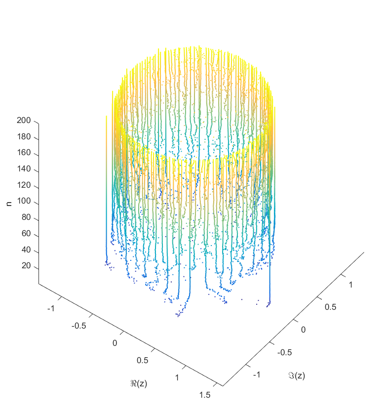
Locations of the zeros of a polynomial with a given sequence of normally distributed coefficients, as a function of degree.
As you add more and more terms to the polynomial the zeros approach the unit circle. Each new term perturbs them a bit: at first they move around a lot as the degree goes up, but they soon stabilize into robust positions (“young” zeros move more than “old” zeros). This seems to be true regardless of whether the coefficients set in “little-endian” or “big-endian” fashion.
But then I decided to move things around: what if the coefficient on the leading term changed? How would the zeros move? I looked at the polynomial where were from some suitable random sequence and could run around . Since the leading coefficient would start and end up back at 1, I knew all zeros would return to their starting position. But in between, would they jump around discontinuously or follow orderly paths?
Continuity is actually guaranteed, as shown by (Harris & Martin 1987). As you change the coefficients continuously, the zeros vary continuously too. In fact, for polynomials without multiple zeros, the zeros vary analytically with the coefficients.
As runs from 0 to the roots move along different orbits. Some end up permuted with each other.
Movement of the zeros of polynomials with random coefficients as the leading coefficient traverses the unit circle. Colour denotes phase, zeros marked by squares.
For low degrees, most zeros participate in a large cycle. Then more and more zeros emerge inside the unit circle and stay mostly fixed as the polynomial changes. As the degree increases they congregate towards the unit circle, while at least one large cycle wraps most of them, often making snaking detours into the zeros near the unit circle and then broad bows outside it.
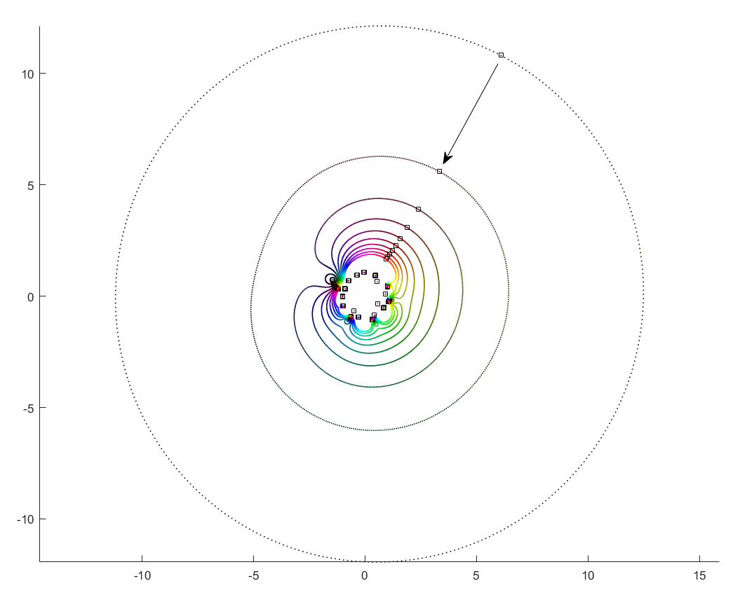
Movement of the zeros of a random degree 100 polynomial.
In the above example, there is a 21-cycle, as well as a 2-cycle around 2 o’clock. The other zeros stay mostly put.
The real question is what determines the cycles? To understand that, we need to change not just the argument but the magnitude of .
Orbits of roots as the magnitude of the leading coefficient increases from zero to one.
What happens if we slowly increase the magnitude of the leading term, letting for a r that increases from zero? It turns out that a new zero of the function zooms in from infinity towards the unit circle. A way of seeing this is to look at the polynomial as : the second term is nonzero and large in most places, so if is small the factor must be large (and opposite) to outweigh it and cause a zero. The exception is of course close to the zeros of , where the perturbation just moves them a tiny bit: there is a counterpart for each of the zeros of among the zeros of . While the new root is approaching from outside, if we play with it will make a turn around the other zeros: it is alone in its orbit, which also encapsulates all the other zeros. Eventually it will start interacting with them, though.
Orbits of roots as the magnitude of the leading coefficient decreases from 100 to one.
If you instead start out with a large leading term, , then the polynomial is essentially and the zeros the n-th roots of . All zeros belong to the same roughly circular orbit, moving together as makes a rotation. But as decreases the shared orbit develops bulges and dents, and some zeros pinch off from it into their own small circles. When does the pinching off happen? That corresponds to when two zeros coincide during the orbit: one continues on the big orbit, the other one settles down to be local. This is the one case where the analyticity of how they move depending on breaks down. They still move continuously, but there is a sharp turn in their movement direction. Eventually we end up in the small term case, with a single zero on a large radius orbit as .
This pinching off scenario also suggests why it is rare to find shared orbits in general: they occur if two zeros coincide but with others in between them (e.g. if we number them along the orbit, , with to separate). That requires a large pinch in the orbit, but since it is overall pretty convex and circle-like this is unlikely.
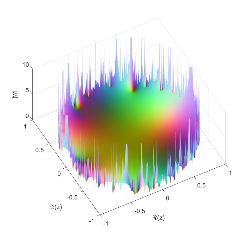
Allowing to run from to 0 and over would cover the entire complex plane (except maybe the origin): for each z, there is some where . This is fairly obviously . This function has a central pole, surrounded by zeros corresponding to the zeros of . The orbits we have drawn above correspond to level sets , and the pinching off to saddle points of this surface. To get a multi-zero orbit several zeros need to be close together enough to cause a broad valley.
Graph of the log-magnitude of f(z), the function mapping a point in the plane to the value of [latex]c_n[/latex] that causes a zero to appear there for [latex]P_n(z)[/latex].
There you have it, a rough theory of dancing zeros.
Recently I chatted with a mathematician friend about generating functions in combinatorics. Normally they are treated as a neat symbolic trick: you have a sequence (typically how many there are of some kind of object of size ), you formally define a function , you derive some constraints on the function, and from this you get a formula for the or other useful data. Convergence does not matter, since this is purely symbolic. We used this in our paper counting tie knots. It is a delightful way of solving recurrence relations or bundle up moments of probability distributions.
I innocently wondered if the function (especially its zeroes and poles) held any interesting information. My friend told me that there was analytic combinatorics: you can actually take seriously as a (complex) function and use the powerful machinery of complex analysis to calculate asymptotic behavior for the from the location and type of the “dominant” singularities. He pointed me at the excellent course notes from a course at Princeton linked to the textbook by Philippe Flajolet and Robert Sedgewick. They show a procedure for taking combinatorial objects, converting them symbolically into generating functions, and then get their asymptotic behavior from the properties of the functions. This is extraordinarily neat, both in terms of efficiency and in linking different branches of math.
Plot of z/(1-z-z^2), the generating function of the Fibonacci numbers. It has poles at (1+sqrt(5))/2 (the dominant pole giving the overall asymptotic growth of Fibonacci numbers) and (1-sqrt(5))/2, which does not contribute much to the asymptotic behavior.
In our case, one can show nearly by inspection that the number of Fink-Mao tie knots grow with the number of moves as , while single tuck tie knots grow as .
Analytic functions behaving badly
The second piece of math I found this weekend was about random Taylor series and lacunary functions.
If where are independent random numbers, what kind of functions do we get? Trying it with complex Gaussian produces a disk of convergence with some nondescript function on the inside.
Plot of function with a Gaussian Taylor series. Color corresponds to stereographic mapping of the complex plane to a sphere, with infinity being white and zeros black. The domain of convergence is the unit circle.
Replacing the complex Gaussian with a real one, or uniform random numbers, or even power-law numbers gives the same behavior. They all seem to have radius 1. This is not just a vanilla disk of convergence (where an analytic function reaches a pole or singularity somewhere on the boundary but is otherwise fine and continuable), but a natural boundary – that is, a boundary so dense with poles or singularities that continuation beyond it is not possible at all.
The locus classicus about random Taylor series is apparently Kahane, J.-P. (1985), Some Random Series of Functions. 2nd ed., Cambridge University Press, Cambridge.
A naive handwave argument is that for we have an exponentially decaying sequence of , so if the have some finite average size and not too divergent variance we should expect convergence, while outside the unit circle any nonzero will allow it to diverge. We can even invoke the Markov inequality to argue that a series would converge if converges. However, this is not correct enough for proper mathematics. One entirely possible Gaussian outcome is or worse. We need to speak of probabilistic convergence.
Andrés E. Caicedo has a good post about how to approach it properly. The “trick” is the awesome Kolmogorov zero-one law that implies that since the radius of convergence depends on the entire series X_n rather than any finite subset (and they are all independent) it will be a constant.
This kind of natural boundary disk of convergence may look odd to beginning students of complex analysis: after all, none of the functions we normally encounter behave like this. Except that this is of course selection bias. If you look at the example series for lacunary functions they all look like fairly reasonable sparse Taylor series like $z+z^4+z^8+z^16+^32+\lddots$. In calculus we are used to worrying that the coefficients in front of the z-terms of a series don’t diminish fast enough: having fewer nonzero terms seems entirely innocuous. But as Hadamard showed, it is enough that the size of the gaps grow geometrically for the function to get a natural boundary (in fact, even denser series do this – for example having just prime powers). The same is true for Fourier series. Weierstrass’ famous continuous but nowhere differentiable function is lacunary (in his 1880 paper on analytic continuation he gives the example of an uncontinuable function). In fact, as Emile Borel found and Steinhardt eventually proved in a stricter sense, in general (“almost surely”) a Taylor series isn’t continuable because of boundaries.
The function [latex]sum_p z^p[/latex], where [latex]p[/latex] runs over the primes.
One could of course try to combine the analytic combinatorics with the lacunary stuff. In a sense a lacunary generating function is a worst case scenario for the singularity-measuring methods used in analytical combinatorics since you get an infinite number of them at a finite and equal distance, and now have to average them together somehow. Intuitively this case seems to correspond to counting something that becomes rarer at a geometric rate or faster. But the Borel-Steinhardt results suggest that even objects that do not become rare could have nasty natural boundaries – if the number were due to something close enough to random we should expect estimating asymptotics to be hard. The funniest example I can think of is the number of roots of Chaitin-style Diophantine equations where for each it is an independent arithmetic fact whether there are any: this is hardcore random, and presumably the exact asymptotic growth rate will be uncomputable both practically and theoretically.

![[\tanh(x),\tanh(y)]](http://s0.wp.com/latex.php?latex=%5B%5Ctanh%28x%29%2C%5Ctanh%28y%29%5D&bg=ffffff&fg=000000&s=0 "[\tanh(x),\tanh(y)]")
![[-1,1]\times [-1,1]](http://s0.wp.com/latex.php?latex=%5B-1%2C1%5D%5Ctimes+%5B-1%2C1%5D&bg=ffffff&fg=000000&s=0 "[-1,1]\times [-1,1]")
![(1/2)+(1/2)[\tanh(|z-1|-1), \tanh(|z+1|-1), \tanh(|z-i|-1)]](http://s0.wp.com/latex.php?latex=%281%2F2%29%2B%281%2F2%29%5B%5Ctanh%28%7Cz-1%7C-1%29%2C+%5Ctanh%28%7Cz%2B1%7C-1%29%2C+%5Ctanh%28%7Cz-i%7C-1%29%5D&bg=ffffff&fg=000000&s=0 "(1/2)+(1/2)[\tanh(|z-1|-1), \tanh(|z+1|-1), \tanh(|z-i|-1)]")


=e^{i\theta} z^n + c_{n-1}z^{n-1}+\ldots+c_1 z + c_0") where
where  were from some suitable random sequence and
  could run around
 ![[0,2\pi]](http://s0.wp.com/latex.php?latex=%5B0%2C2%5Cpi%5D&bg=ffffff&fg=000000&s=0 "[0,2\pi]") . Since the leading coefficient would start and end up back at 1, I knew all zeros would return to their starting position. But in between, would they jump around discontinuously or follow orderly paths?
. Since the leading coefficient would start and end up back at 1, I knew all zeros would return to their starting position. But in between, would they jump around discontinuously or follow orderly paths? the roots move along different orbits. Some end up permuted with each other.
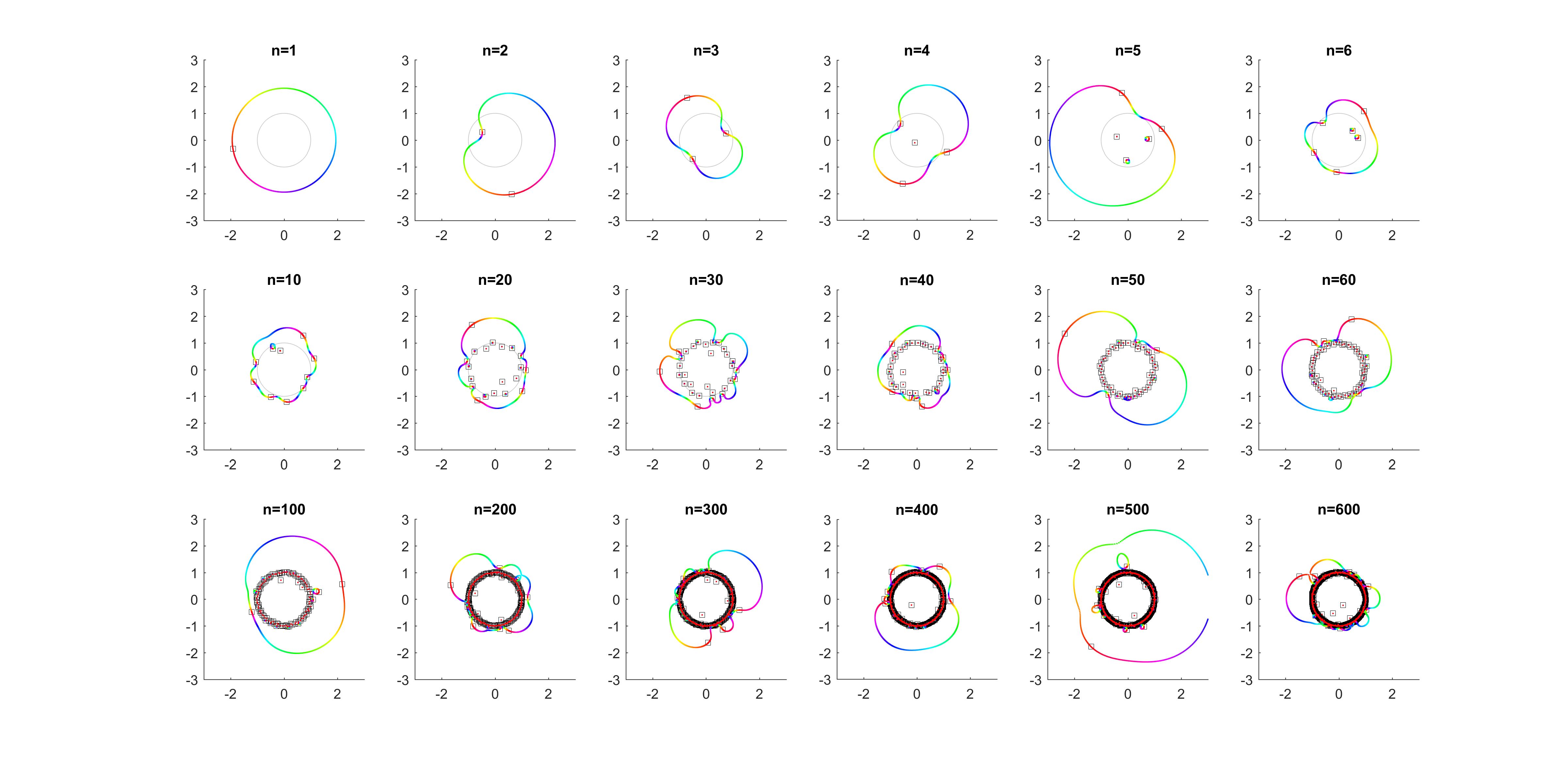
 .
.
 for a r that increases from zero? It turns out that a new zero of the function zooms in from infinity towards the unit circle. A way of seeing this is to look at the polynomial as
  = c_n z^n + P_{n-1}(z)") : the second term is nonzero and large in most places, so if
: the second term is nonzero and large in most places, so if  factor must be large (and opposite) to outweigh it and cause a zero. The exception is of course close to the zeros of
 ") , where the perturbation just moves them a tiny bit: there is a counterpart for each of the
, where the perturbation just moves them a tiny bit: there is a counterpart for each of the  zeros of
 ") . While the new root is approaching from outside, if we play with
. While the new root is approaching from outside, if we play with 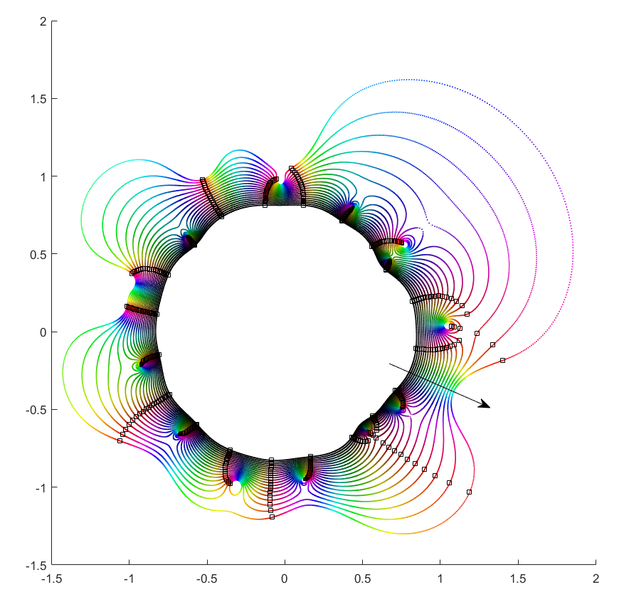
 , then the polynomial is essentially
 ![P_n(z)=c_nz^n+[\mathrm{small stuff}]](http://s0.wp.com/latex.php?latex=P_n%28z%29%3Dc_nz%5En%2B%5B%5Cmathrm%7Bsmall+stuff%7D%5D&bg=ffffff&fg=000000&s=0 "P_n(z)=c_nz^n+[\mathrm{small stuff}]") and the zeros the n-th roots of
and the zeros the n-th roots of ![-[\mathrm{small stuff}]/c_n](http://s0.wp.com/latex.php?latex=-%5B%5Cmathrm%7Bsmall+stuff%7D%5D%2Fc_n&bg=ffffff&fg=000000&s=0 "-[\mathrm{small stuff}]/c_n") . All zeros belong to the same roughly circular orbit, moving together as
. All zeros belong to the same roughly circular orbit, moving together as  decreases the shared orbit develops bulges and dents, and some zeros pinch off from it into their own small circles. When does the pinching off happen? That corresponds to when two zeros coincide during the orbit: one continues on the big orbit, the other one settles down to be local. This is the one case where the analyticity of how they move depending on
  .
. , with
  to
to  separate). That requires a large pinch in the orbit, but since it is overall pretty convex and circle-like this is unlikely.
 to 0 and
  . This is fairly obviously
  = -P_{n-1}(z)/z^n") . This function has a central pole, surrounded by zeros corresponding to the zeros of
. This function has a central pole, surrounded by zeros corresponding to the zeros of |=\mathrm{const}") , and the pinching off to saddle points of this surface. To get a multi-zero orbit several zeros need to be close together enough to cause a broad valley.
, and the pinching off to saddle points of this surface. To get a multi-zero orbit several zeros need to be close together enough to cause a broad valley.
 ), you formally define a function
 =\sum_{n=0}^\infty a_n z^n") , you derive some constraints on the function, and from this you get a formula for the
, you derive some constraints on the function, and from this you get a formula for the ") seriously as a (complex) function and use the powerful machinery of complex analysis to calculate asymptotic behavior for the
seriously as a (complex) function and use the powerful machinery of complex analysis to calculate asymptotic behavior for the 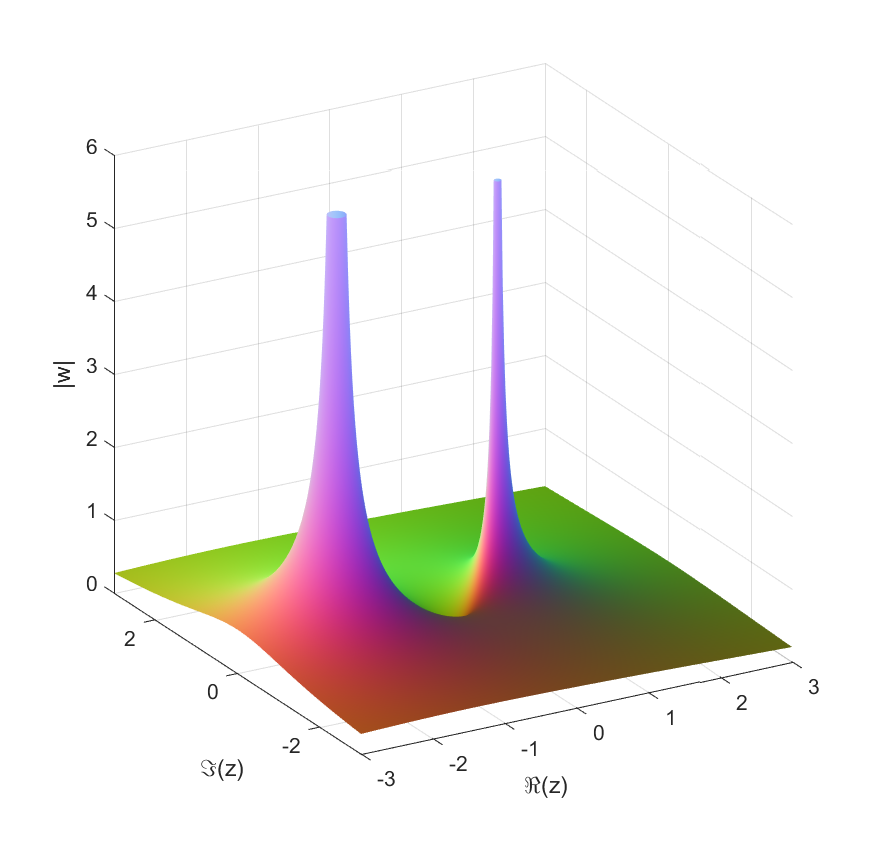
 , while single tuck tie knots grow as
  .
.=\sum_{n=0}^\infty X_n z^n") where
where  are independent random numbers, what kind of functions do we get? Trying it with complex Gaussian
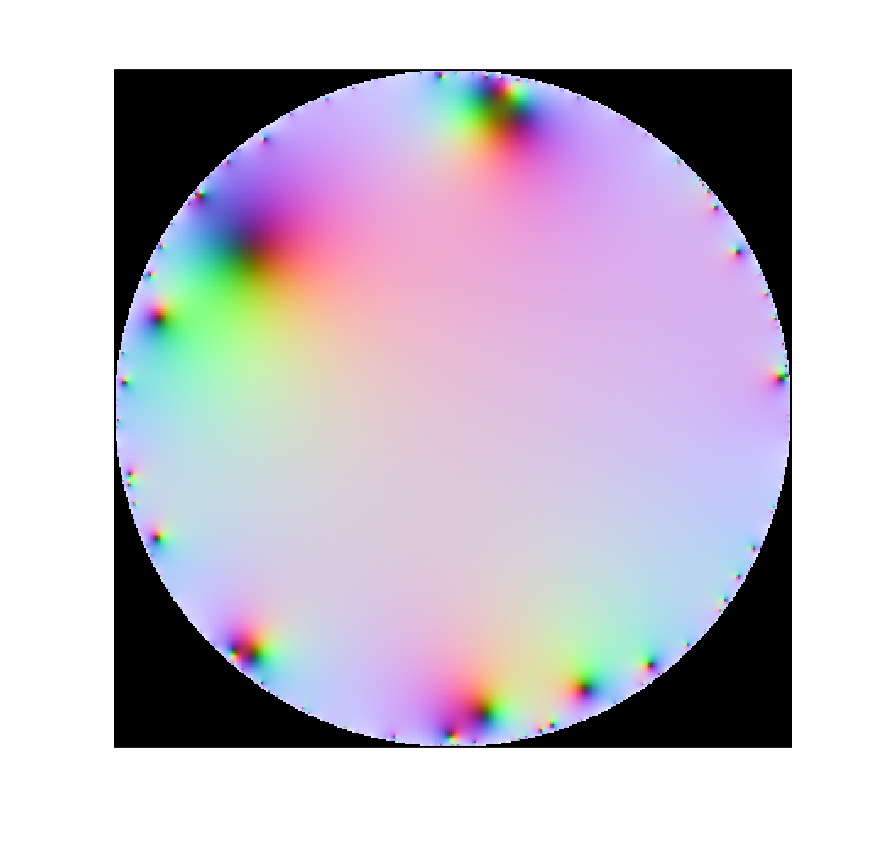
 we have an exponentially decaying sequence of
 ") and not too divergent variance we should expect convergence, while outside the unit circle any nonzero
and not too divergent variance we should expect convergence, while outside the unit circle any nonzero  \leq E(X)/t") to argue that a series
to argue that a series ") would converge if
would converge if /n") converges. However, this is not correct enough for proper mathematics. One entirely possible Gaussian outcome is
converges. However, this is not correct enough for proper mathematics. One entirely possible Gaussian outcome is  or worse. We need to speak of probabilistic convergence.
 of an uncontinuable function). In fact,