roots

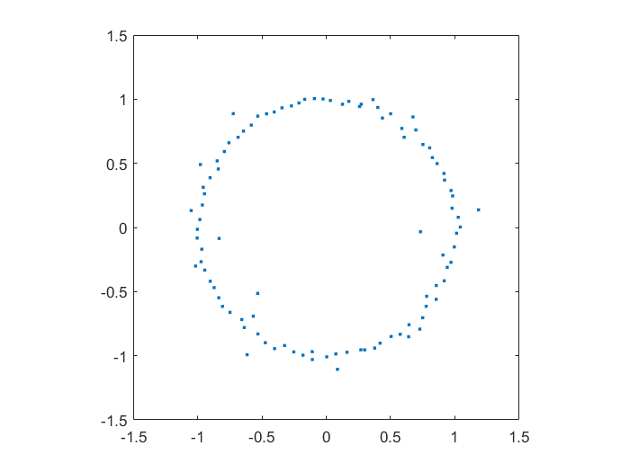
Playing with Matlab, I plotted the location of the zeros of a polynomial with normally distributed coefficients in the complex plane. It was nearly a circle:

Zeros in the complex plane of a 100-degree polynomial with normally distributed random coefficients. — Zeros of a 100-degree polynomial with normally distributed random coefficients.

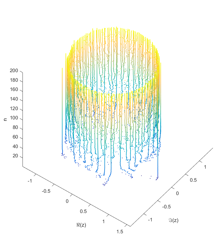
This did not surprise me that much, since I have already toyed with the distribution of zeros of polynomials with coefficients in {-1,0,+1}, producing some neat distributions close to the unit circle (see also John Baez). A quick google found (Hughes & Nikeghbali 2008): under very general circumstances polynomial zeros tend towards the unit circle. One can heuristically motivate it in a lot of ways.

Locations of the zeros of a polynomial with a given sequence of normally distributed coefficients, as a function of degree.

As you add more and more terms to the polynomial the zeros approach the unit circle. Each new term perturbs them a bit: at first they move around a lot as the degree goes up, but they soon stabilize into robust positions (“young” zeros move more than “old” zeros). This seems to be true regardless of whether the coefficients set in “little-endian” or “big-endian” fashion.

But then I decided to move things around: what if the coefficient on the leading term changed? How would the zeros move? I looked at the polynomial $P_\theta(z)=e^{i\theta} z^n + c_{n-1}z^{n-1}+\ldots+c_1 z + c_0$ where $c_i$ were from some suitable random sequence and $\theta$ could run around $[0,2\pi]$ . Since the leading coefficient would start and end up back at 1, I knew all zeros would return to their starting position. But in between, would they jump around discontinuously or follow orderly paths?

Continuity is actually guaranteed, as shown by (Harris & Martin 1987). As you change the coefficients continuously, the zeros vary continuously too. In fact, for polynomials without multiple zeros, the zeros vary analytically with the coefficients.

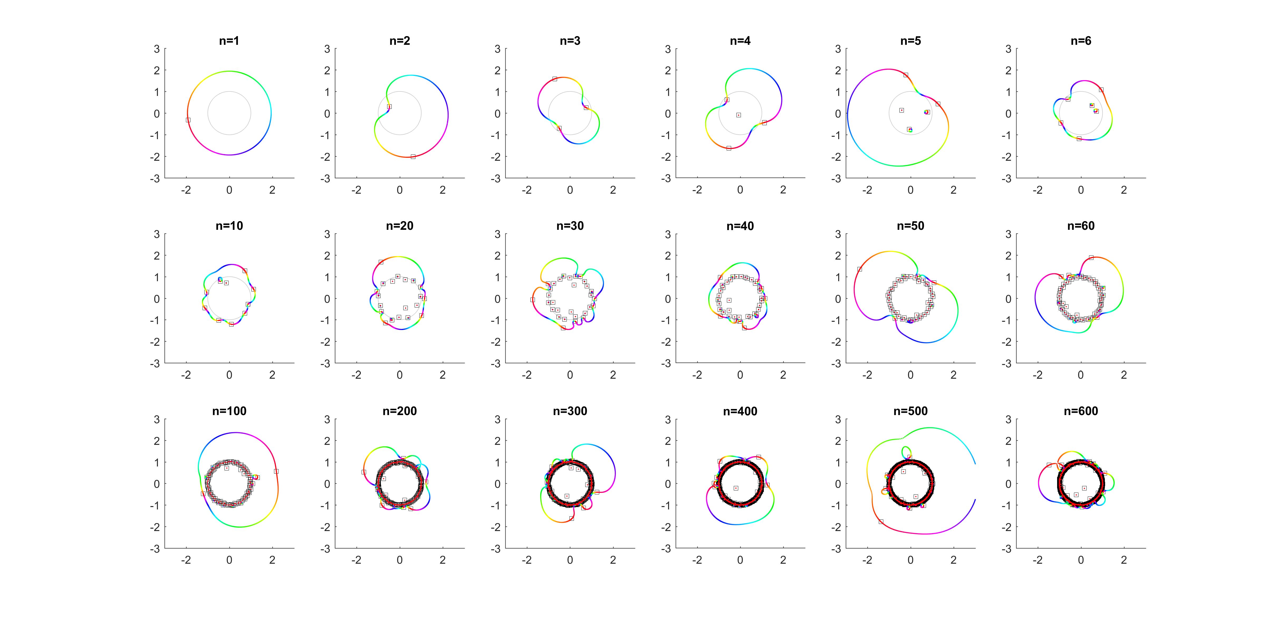
As $\theta$ runs from 0 to $2\pi$ the roots move along different orbits. Some end up permuted with each other.

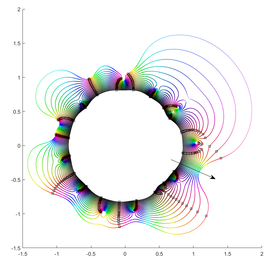
Movement of the zeros of polynomials with random coefficients as the leading coefficient traverses the unit circle. Colour denotes phase, zeros marked by squares.

For low degrees, most zeros participate in a large cycle. Then more and more zeros emerge inside the unit circle and stay mostly fixed as the polynomial changes. As the degree increases they congregate towards the unit circle, while at least one large cycle wraps most of them, often making snaking detours into the zeros near the unit circle and then broad bows outside it.

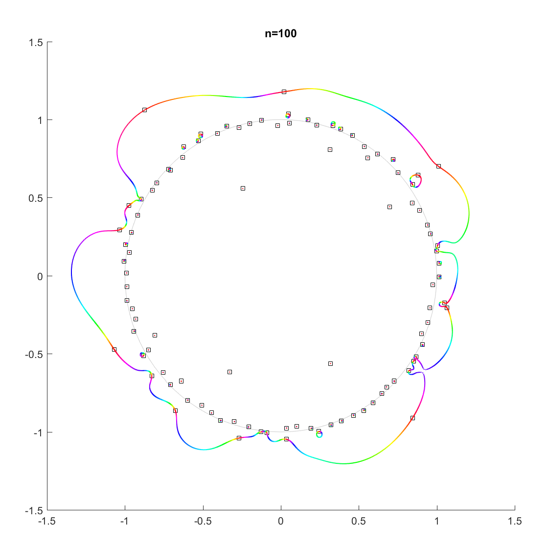
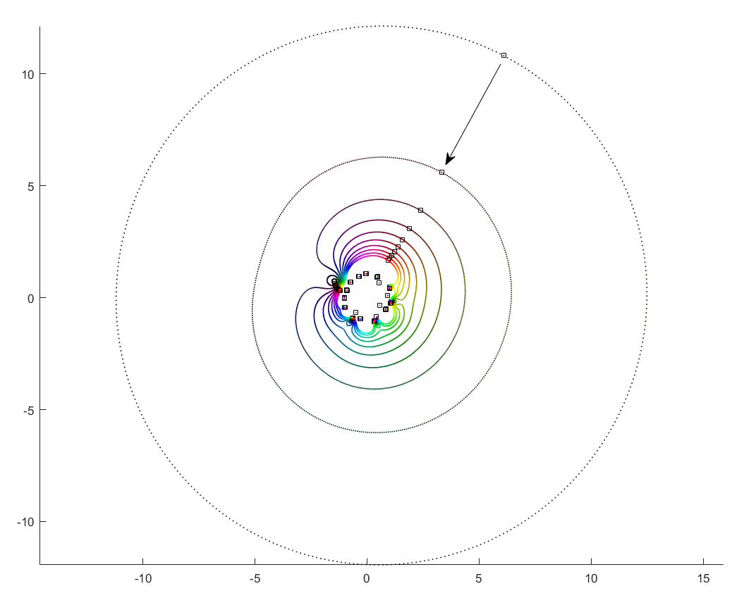
Movement of the zeros of a random degree 100 polynomial.

In the above example, there is a 21-cycle, as well as a 2-cycle around 2 o’clock. The other zeros stay mostly put.

The real question is what determines the cycles? To understand that, we need to change not just the argument but the magnitude of $c_n$ .

Orbits of roots as the magnitude of the leading coefficient increases from zero to one.

What happens if we slowly increase the magnitude of the leading term, letting $c_n = re^{i\theta}$ for a r that increases from zero? It turns out that a new zero of the function zooms in from infinity towards the unit circle. A way of seeing this is to look at the polynomial as $P_n(z) = c_n z^n + P_{n-1}(z)$ : the second term is nonzero and large in most places, so if $c_n$ is small the $z^n$ factor must be large (and opposite) to outweigh it and cause a zero. The exception is of course close to the zeros of $P_{n-1}(z)$ , where the perturbation just moves them a tiny bit: there is a counterpart for each of the $n-1$ zeros of $P_{n-1}(z)$ among the zeros of $P_{n}(z)$ . While the new root is approaching from outside, if we play with $\theta$ it will make a turn around the other zeros: it is alone in its orbit, which also encapsulates all the other zeros. Eventually it will start interacting with them, though.

Orbits of roots as the magnitude of the leading coefficient decreases from 100 to one.

If you instead start out with a large leading term, $|c_n| \gg |c_i|$ , then the polynomial is essentially $P_n(z)=c_nz^n+[\mathrm{small stuff}]$ and the zeros the n-th roots of $-[\mathrm{small stuff}]/c_n$ . All zeros belong to the same roughly circular orbit, moving together as $\theta$ makes a rotation. But as $|c_n|$ decreases the shared orbit develops bulges and dents, and some zeros pinch off from it into their own small circles. When does the pinching off happen? That corresponds to when two zeros coincide during the orbit: one continues on the big orbit, the other one settles down to be local. This is the one case where the analyticity of how they move depending on $c_n$ breaks down. They still move continuously, but there is a sharp turn in their movement direction. Eventually we end up in the small term case, with a single zero on a large radius orbit as $|c_n| \rightarrow 0$ .

This pinching off scenario also suggests why it is rare to find shared orbits in general: they occur if two zeros coincide but with others in between them (e.g. if we number them along the orbit, $z_1=z_k$ , with $z_2$ to $z_{k-1}$ separate). That requires a large pinch in the orbit, but since it is overall pretty convex and circle-like this is unlikely.

Allowing $|c_n|$ to run from $\infty$ to 0 and $\theta$ over $[0,2\pi]$ would cover the entire complex plane (except maybe the origin): for each z, there is some $c_n$ where $c_nz^n+\ldots+c_1z+c_0=0$ . This is fairly obviously $c_n = f(z) = -P_{n-1}(z)/z^n$ . This function has a central pole, surrounded by zeros corresponding to the zeros of $P_{n-1}(z)$ . The orbits we have drawn above correspond to level sets $|f(z)|=\mathrm{const}$ , and the pinching off to saddle points of this surface. To get a multi-zero orbit several zeros need to be close together enough to cause a broad valley.