Apropos Newton’s method in the complex plane, what happens when the degree of the polynomial goes to infinity?
Towards infinity
Obviously there will be more zeros, so there will be more attractors and we should expect the boundaries of the basins of attraction to become messier. But it is not entirely clear where the action will be, so it would be useful to compress the entire complex plane into a convenient square.
How do you depict the entire complex plane? While I have always liked the Riemann sphere here I tried mapping to . The origin is unchanged, and infinity becomes the edges of the square . This is not a conformal map, so things will get squished near the edges.
For color, I used to map complex coordinates to RGB. This makes the color depend on the distance to 1, -1 and i, making infinity white and zero some drab color (the -1 terms at the end determines the overall color range).
Here is the animated result:
What is going on? As I scale up the size of the leading term from zero, the root created by adding that term moves in from infinity towards the center, making the new basin of attraction grow. This behavior has been described in this post on dancing zeros. The zeros also tend to cluster towards the unit circle, crowding together and distributing themselves evenly. That distribution is the reason for the the colorful “flowers” that surround white spots (poles of the Newton formula, corresponding to zeros of the derivative of the polynomial). The central blob is just the attractor of the most “solid” zero, corresponding to the linear and constant terms of the polynomial.
The jostling is amusing: it looks like the roots do repel each other. This is presumably because close roots require a sharp turn of the function, but the “turning radius” is set by the coefficients that tend to be of order unity. Getting degenerate roots requires coefficients to be in a set of measure zero, so it is rare. Near-degenerate roots exist in a positive measure set surrounding that set, but it is still “small” compared to the general case.
At infinity
So what happens if we let the degree go to infinity? As I previously mentioned, the generic behaviour of where is independent random numbers is a lacunary function. So we should not expect anything outside the unit circle. Inside the circle there will be poles, so there will be copies of the undefined outside region (because of Great Picard’s Theorem (meromorphic version)). Since the function is analytic these copies will be conformal mappings of the exterior and hence roughly circular. There will also be zeros, and these will have their own basins of attraction. A few of the central ones dominate, but there is an infinite number of attractors as we approach the circular border which is crammed with poles and zeros.
Since we now know we will only deal with the unit disk, we can avoid transforming the entire plane and enjoy the results:
Attractors for random 10,000-degree polynomial.Attractors for random 10,000-degree polynomial.
What happens here is that the white regions represents places where points get mapped onto the undefined outside, while the colored fractal regions are the attraction basins for the zeros. And between them there is a truly wild boundary. In the vanilla fractal every point on the boundary is a meeting point of the three basins, a tri-point. Here there is an infinite number of attractors: the boundary consists of points where an infinite number of different attractors meet.
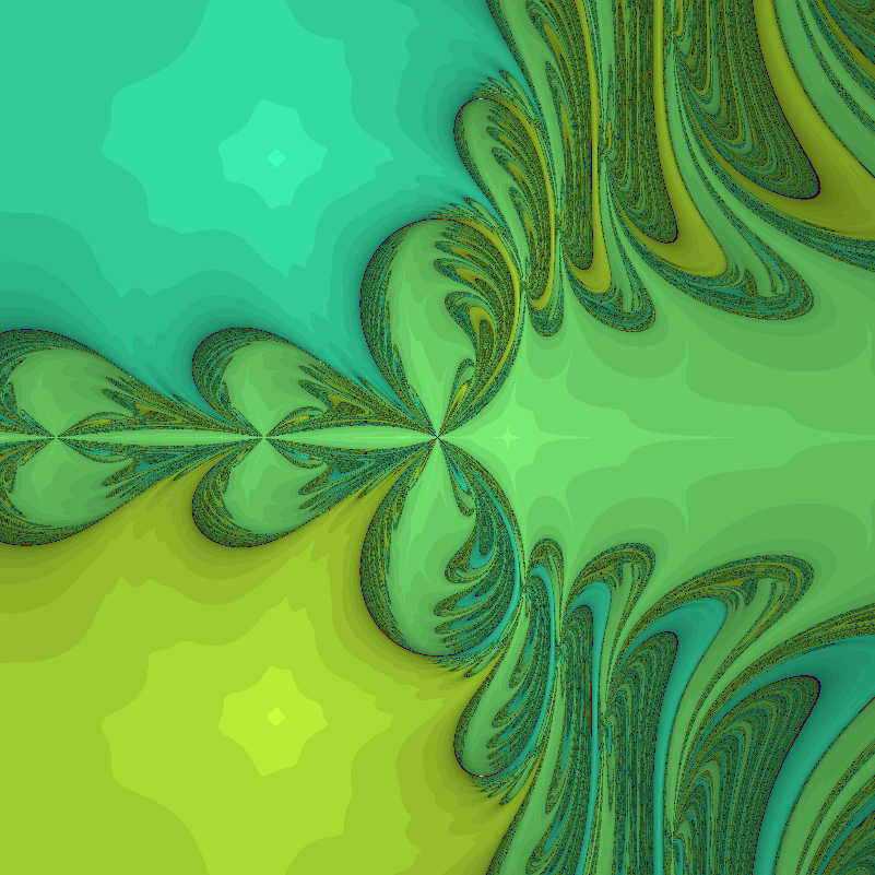
But what if we looked at real functions? If we use a single function the zeros will typically form a curve in the plane. In order to get discrete zeros we typically need to have two functions to produce a zero set. We can think of it as a map from R2 to R2 where the x’es are 2D vectors. In this case Newton’s method turns into solving the linear equation system where is the Jacobian matrix () and now denotes the n’th iterate.
The simplest case of nontrivial dynamics of the method is for third degree polynomials, and we want the x- and y-directions to interact a bit, so a first try is . Below is a plot of the first and second components (red and green), as well as a blue plane for zero values. The zeros of the function are the three points where red, green and blue meet.
We have three zeros, one at , one at , and one at The middle one has a region of troublesomely similar function values – the red and green surfaces are tangent there.
Plot of x^3-x-y (red), y^3-x-y (green) and z=0 (blue). The zeros found using Newton’s method are the points where red, green and blue meet.
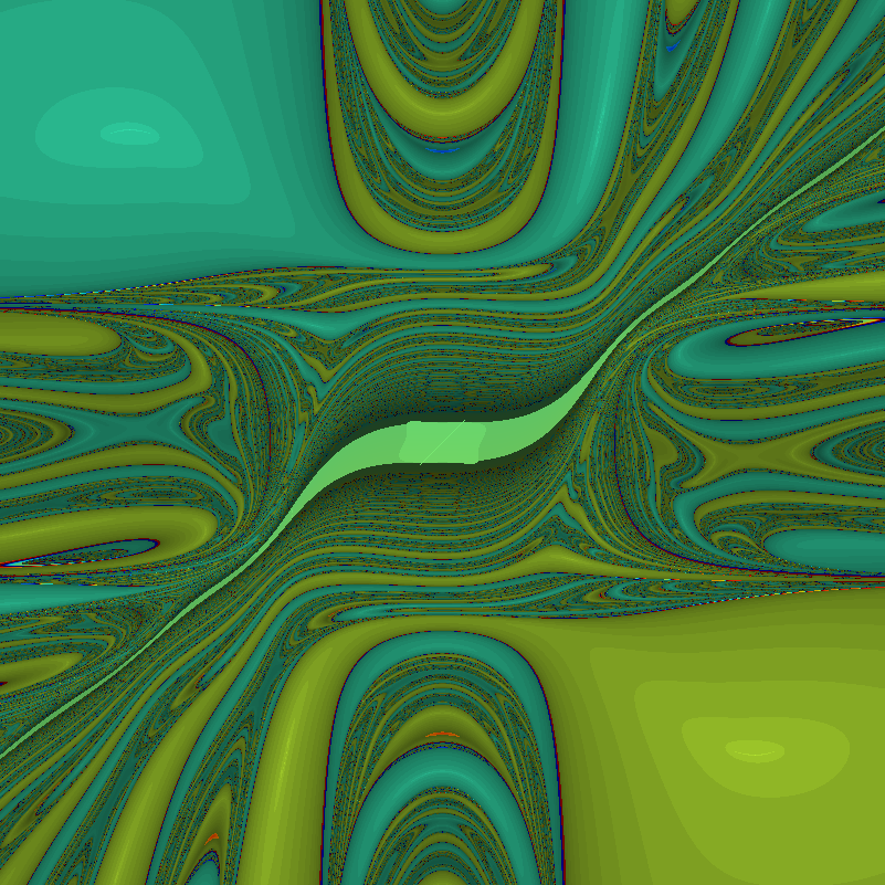
The resulting fractal has a decided modernist bent to it, all hyperbolae and swooshes:
Behavior of Newton’s method in 2D for F=[x^3-x-y, y^3-x-y]. Color denotes value of x+y, with darkening for slow convergence.The troublesome region shows up, as well as the red and blue regions where iterates run off to large or small values: the three roots are green shades.
Why is the style modernist?
In complex iterations you typically multiply with complex numbers, and if they have an imaginary component (they better have, to be complex!) that introduces a rotation or twist. Hence baroque filaments are ubiquitous, and you get the typical complex “style”.
But here we are essentially multiplying with a real matrix. For a real 2×2 matrix to be a rotation matrix it has to have a pair of imaginary eigenvalues, and for it to at least twist things around the trace needs to be small enough compared to the determinant so that there are complex eigenvalues: (where and if the matrix has the usual form). So if the trace and determinant are randomly chosen, we should expect a majority of cases to be non-rotational.
Moreover, in this particular case, the Jacobian tends to be diagonally dominant (quadratic terms on the diagonal) and that makes the inverse diagonally dominant too: the trace will be big, and hence the chance of seeing rotation goes down even more. The two “knots” where a lot of basins of attraction come together are the points where the trace does vanish, but since the Jacobian is also symmetric there will not be any rotation anyway. Double guarantee.
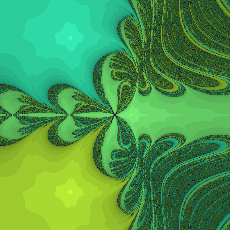
Can we make a twisty real Newton fractal? If we start with a vanilla rotation matrix and try to find a function that produces it the simplest case is . This is of course just a rotation by the angle theta, and it does not have very interesting zeros.
To get something fractal we need more zeros, and a few zeros in the derivatives too (why? because they cause iterates to be thrown away far from where they were, ensuring a complicated structure of the basin boundaries). One attempt is . The result is fun, but still far from baroque:
Basins of attraction for Netwon’s method of twisted cubic. theta=1.Basins of attraction for Netwon’s method of twisted cubic. theta=0.1.
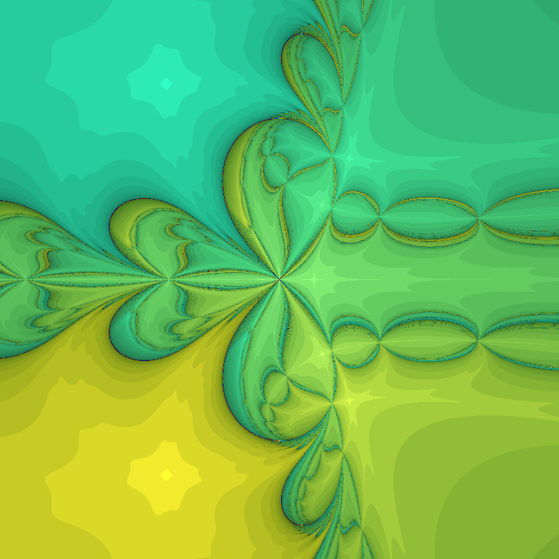
The problem might be that the twistiness is not changing. So we can make to make the dynamics even more complex:
Basins of attraction with rotation proportional to x.
Quite lovely, although still not exactly what I wanted (sounds like a Christmas present).
Back to the classics?
It might be easier just to hide the complex dynamics in an apparently real function like (which produces the archetypal Newton fractal).
Newton fractal for F=[x^3-3xy^2-1, 3x^2y-y^3]. Red and blue circles mark regions where iterates venture far from the origin.It is interesting to see how much perturbing it causes a modernist shift. If we use , then for we get:
Perturbed z^3-1 Newton iteration, epsilon=1.
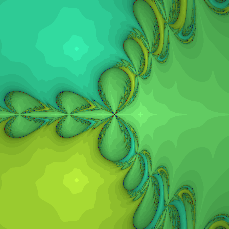
As we make the function more perturbed, it turns more modernist, undergoing a topological crisis for epsilon between 3.5 and 4:
Perturbed z^3-1 Newton iteration, epsilon=2.Perturbed z^3-1 Newton iteration, epsilon=3.Perturbed z^3-1 Newton iteration, epsilon=3.5.Perturbed z^3-1 Newton iteration, epsilon=4.
In the end, we can see that the border between classic baroque complex fractals and the modernist swooshy real fractals is fuzzy. Or, indeed, fractal.
Robin Hanson mentions that some people take him to task for working on one scenario (WBE) that might not be the most likely future scenario (“standard AI”); he responds by noting that there are perhaps 100 times more people working on standard AI than WBE scenarios, yet the probability of AI is likely not a hundred times higher than WBE. He also notes that there is a tendency for thinkers to clump onto a few popular scenarios or issues. However:
In addition, due to diminishing returns, intellectual attention to future scenarios should probably be spread out more evenly than are probabilities. The first efforts to study each scenario can pick the low hanging fruit to make faster progress. In contrast, after many have worked on a scenario for a while there is less value to be gained from the next marginal effort on that scenario.
This is very similar to my own thinking about research effort. Should we focus on things that are likely to pan out, or explore a lot of possibilities just in case one of the less obvious cases happens? Given that early progress is quick and easy, we can often get a noticeable fraction of whatever utility the topic has by just a quick dip. The effective altruist heuristic of looking at neglected fields also is based on this intuition.
A model
But under what conditions does this actually work? Here is a simple model:
There are possible scenarios, one of which () will come about. They have probability . We allocate a unit budget of effort to the scenarios: . For the scenario that comes about, we get utility (diminishing returns).
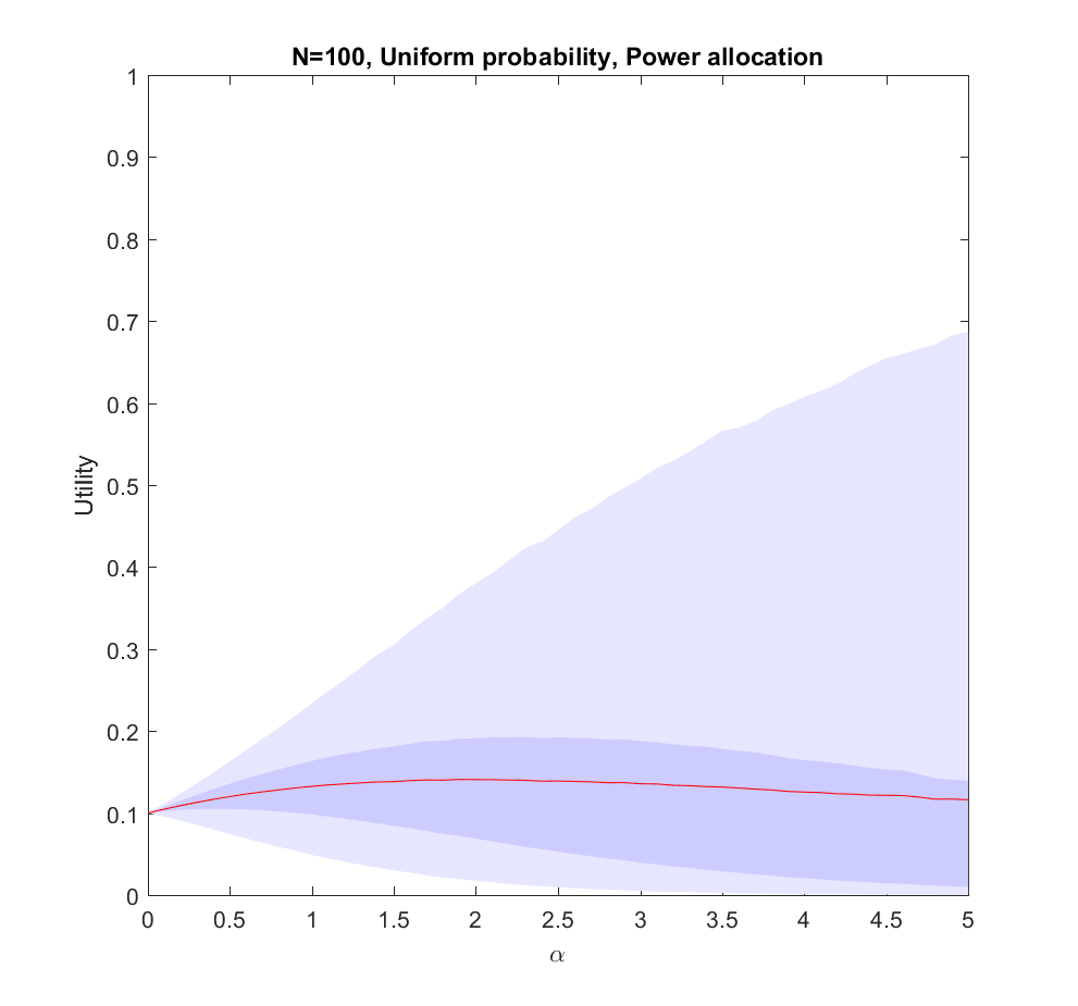
Here is what happens if we allocate proportional to a power of the scenarios, . corresponds to even allocation, 1 proportional to the likelihood, >1 to favoring the most likely scenarios. In the following I will run Monte Carlo simulations where the probabilities are randomly generated each instantiation. The outer bluish envelope represents the 95% of the outcomes, the inner ranges from the lower to the upper quartile of the utility gained, and the red line is the expected utility.
Utility of allocating effort as a power of the probability of scenarios. Red line is expected utility, deeper blue envelope is lower and upper quartiles, lighter blue 95% interval.
This is the case: we have two possible scenarios with probability and (where is uniformly distributed in [0,1]). Just allocating evenly gives us utility on average, but if we put in more effort on the more likely case we will get up to 0.8 utility. As we focus more and more on the likely case there is a corresponding increase in variance, since we may guess wrong and lose out. But 75% of the time we will do better than if we just allocated evenly. Still, allocating nearly everything to the most likely case means that one does lose out on a bit of hedging, so the expected utility declines slowly for large .
Utility of allocating effort as a power of the probability of scenarios. Red line is expected utility, deeper blue envelope is lower and upper quartiles, lighter blue 95% interval. 100 possible scenarios, with uniform probability on the simplex.
The case (where the probabilities are allocated based on a flat Dirichlet distribution) behaves similarly, but the expected utility is smaller since it is less likely that we will hit the right scenario.
What is going on?
This doesn’t seem to fit Robin’s or my intuitions at all! The best we can say about uniform allocation is that it doesn’t produce much regret: whatever happens, we will have made some allocation to the possibility. For large N this actually works out better than the directed allocation for a sizable fraction of realizations, but on average we get less utility than betting on the likely choices.
The problem with the model is of course that we actually know the probabilities before making the allocation. In reality, we do not know the likelihood of AI, WBE or alien invasions. We have some information, and we do have priors (like Robin’s view that ), but we are not able to allocate perfectly. A more plausible model would give us probability estimates instead of the actual probabilities.
We know nothing
Let us start by looking at the worst possible case: we do not know what the true probabilities are at all. We can draw estimates from the same distribution – it is just that they are uncorrelated with the true situation, so they are just noise.
Utility of allocating effort as a power of the probability of scenarios, but the probabilities are just random guesses. Red line is expected utility, deeper blue envelope is lower and upper quartiles, lighter blue 95% interval. 100 possible scenarios, with uniform probability on the simplex.
In this case uniform distribution of effort is optimal. Not only does it avoid regret, it has a higher expected utility than trying to focus on a few scenarios (). The larger N is, the less likely it is that we focus on the right scenario since we know nothing. The rationality of ignoring irrelevant information is pretty obvious.
Note that if we have to allocate a minimum effort to each investigated scenario we will be forced to effectively increase our above 0. The above result gives the somewhat optimistic conclusion that the loss of utility compared to an even spread is rather mild: in the uniform case we have a pretty low amount of effort allocated to the winning scenario, so the low chance of being right in the nonuniform case is being balanced by having a slightly higher effort allocation on the selected scenarios. For high there is a tail of rare big “wins” when we hit the right scenario that drags the expected utility upwards, even though in most realizations we bet on the wrong case. This is very much the hedgehog predictor story: ocasionally they have analysed the scenario that comes about in great detail and get intensely lauded, despite looking at the wrong things most of the time.
We know a bit
We can imagine that knowing more should allow us to gradually interpolate between the different results: the more you know, the more you should focus on the likely scenarios.
Optimal alpha as a function of how much information we have about the true probabilities (noise due to Monte Carlo and discrete steps of alpha). N=2 (N=100 looks similar).
If we take the mean of the true probabilities with some randomly drawn probabilities (the “half random” case) the curve looks quite similar to the case where we actually know the probabilities: we get a maximum for . In fact, we can mix in just a bit () of the true probability and get a fairly good guess where to allocate effort (i.e. we allocate effort as where is uncorrelated noise probabilities). The optimal alpha grows roughly linearly with , in this case.
We learn
Adding a bit of realism, we can consider a learning process: after allocating some effort to the different scenarios we get better information about the probabilities, and can now reallocate. A simple model may be that the standard deviation of noise behaves as where is the effort placed in exploring the probability of scenario . So if we begin by allocating uniformly we will have noise at reallocation of the order of . We can set , where is some constant denoting how tough it is to get information. Putting this together with the above result we get . After this exploration, now we use the remaining effort to work on the actual scenarios.
Expected utility as a function of amount of probability-estimating effort (gamma) for C=1 (hard to update probabilities), C=0.1 and C=0.01 (easy to update). N=100.
This is surprisingly inefficient. The reason is that the expected utility declines as and the gain is just the utility difference between the uniform case and optimal , which we know is pretty small. If C is small (i.e. a small amount of effort is enough to figure out the scenario probabilities) there is an optimal nonzero . This optimum decreases as C becomes smaller. If C is large, then the best approach is just to spread efforts evenly.
Conclusions
So, how should we focus? These results suggest that the key issue is knowing how little we know compared to what can be known, and how much effort it would take to know significantly more.
If there is little more that can be discovered about what scenarios are likely, because our state of knowledge is pretty good, the world is very random, or improving knowledge about what will happen will be costly, then we should roll with it and distribute effort either among likely scenarios (when we know them) or spread efforts widely (when we are in ignorance).
If we can acquire significant information about the probabilities of scenarios, then we should do it – but not overdo it. If it is very easy to get information we need to just expend some modest effort and then use the rest to flesh out our scenarios. If it is doable but costly, then we may spend a fair bit of our budget on it. But if it is hard, it is better to go directly on the object level scenario analysis as above. We should not expect the improvement to be enormous.
Here I have used a square root diminishing return model. That drives some of the flatness of the optima: had I used a logarithm function things would have been even flatter, while if the returns diminish more mildly the gains of optimal effort allocation would have been more noticeable. Clearly, understanding the diminishing returns, number of alternatives, and cost of learning probabilities better matters for setting your strategy.
In the case of future studies we know the number of scenarios are very large. We know that the returns to forecasting efforts are strongly diminishing for most kinds of forecasts. We know that extra efforts in reducing uncertainty about scenario probabilities in e.g. climate models also have strongly diminishing returns. Together this suggests that Robin is right, and it is rational to stop clustering too hard on favorite scenarios. Insofar we learn something useful from considering scenarios we should explore as many as feasible.
In Scott Alexander’s kabbalistic sf story Unsong, the archangel Uriel works on a problem while other things are going on in heaven:
All the angels listened in rapt attention except Uriel, who was sort of half-paying attention while trying to balance several twelve-dimensional shapes on top of each other.
…
There was utter silence throughout the halls of Heaven, except a brief curse as Uriel’s hyperdimensional tower collapsed on itself and he picked up the pieces to try to rebuild it.
…
A great clamor arose from all the heavenly hosts, save Uriel, who took advantage of the brief lapse to conjure a parchment and pen and start working on a proof about the optimal configuration of twelve-dimensional shapes.
This got me thinking about the stability of stacking polytopes. That seemed complicated (I am no archangel) so I started toying with the stability of polytopes on a flat surface.
(Terminology note: I will consistently use “face” to denote the D-1 dimensional elements that bound the polytope, although “facet” is in some use.)
A face of a 3D polyhedron is stable if the polyhedron can rest on it without tipping over. This means that the projection of the center of mass onto the plane containing the face is inside the polygon. The platonic polyhedra are stable on all faces, but it is not hard to make a few faces unstable by moving a vertex far away from the center. A polyhedron has at least one stable face (if it did not, it would be a perpetual motion device: every tip will move the center of mass downwards, but there is a bound on how low it can go. A uni-stable or monostatic polyhedron has just one stable face. It is an unsolved problem what the simplest uni-stable 3D polyhedron is, with the current record 14 faces. Also, it seems unclear whether there are monostatic simplices in dimension 9 (they exist in 10 or more dimensions, but not in 8 or fewer).
So, how many faces of a polytope will typically be unstable?
I wrote a Matlab script to generate random convex polytopes by selecting N points randomly on the surface of a D-dimensional sphere and calculating their convex hull. Using a Delaunay decomposition I can split them into simplices, which allow me to calculate the center of mass. The center of mass of a simplex is just the average of the corners , and the center of mass of the polyhedron is just the sum of the simplex centers of mass weighted by their volumes: . The volume of a simplex is where , the matrix made by sticking together the coordinate vectors of a simplex. Once we know this we can project the center of mass onto the plane of a face by finding its nullspace (the higher dimensional counterpart to a normal) . Finally, to check whether the projection is inside the face, we can look at the matrix A where each column is the coordinates of one of the faces minus and the final row just ones, and solve for Ax=b where b is zero except for a one in the last row (I found this neat algorithm due to elisbben on stack overflow). If the answer vector is all positive, then the point is inside the face. Repeat for all the faces.
Whew. This math is of course really simple to do in Matlab.
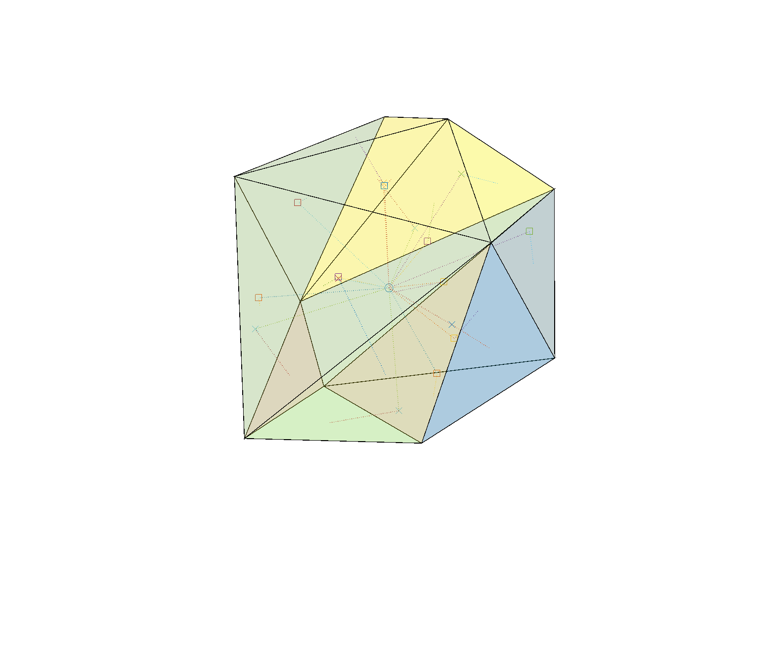
Stable (yellow) and unstable (blue) faces of random polyhedron.Stability of random polyhedron. The center of mass is marked by a circle. It is projected along the dotted lines into the plane of each face, marked with a square (if inside the face and hence a stable face) or a cross (if outside the face, which is hence unstable). A dotted line connects the projection points to the center of their face.
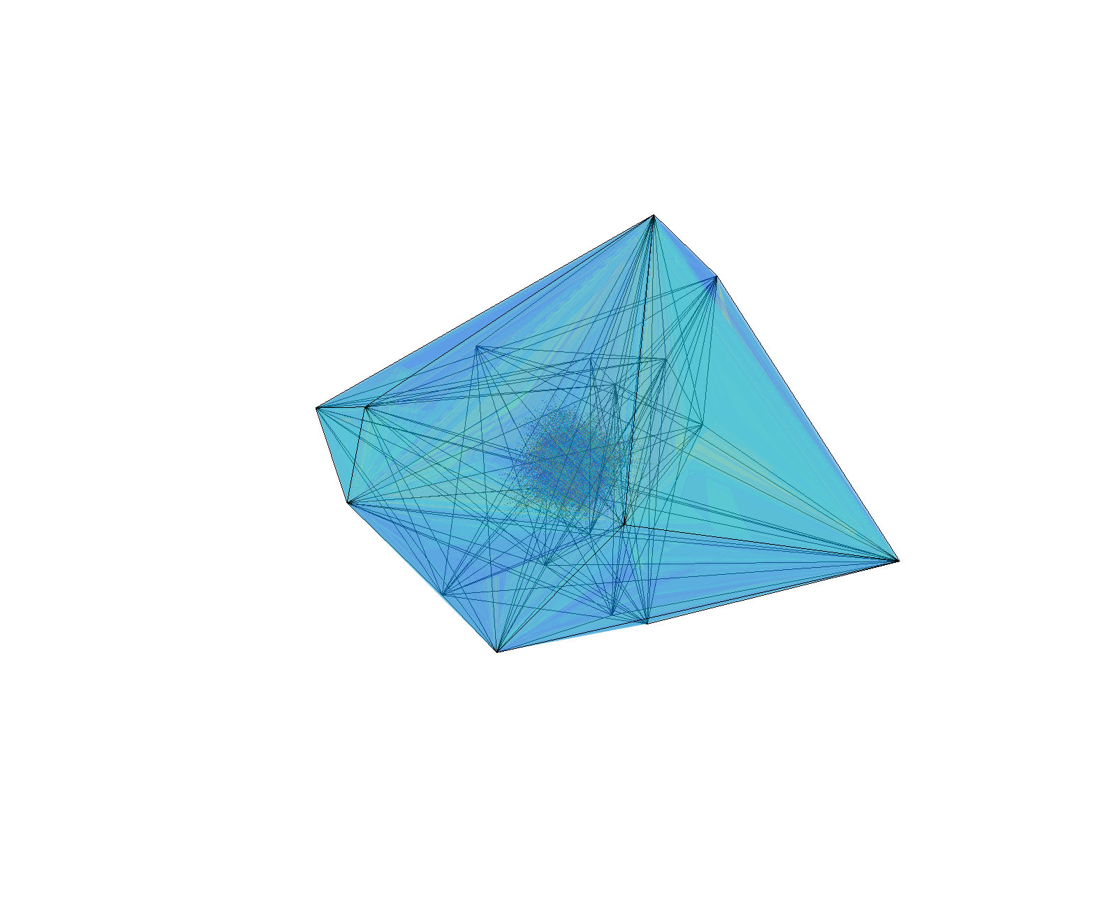
The 12 dimensional case is a bit messier:
Projection of a 12D polytope with 20 vertices. Each of the 2777 faces is a 11 dimensional simplex.
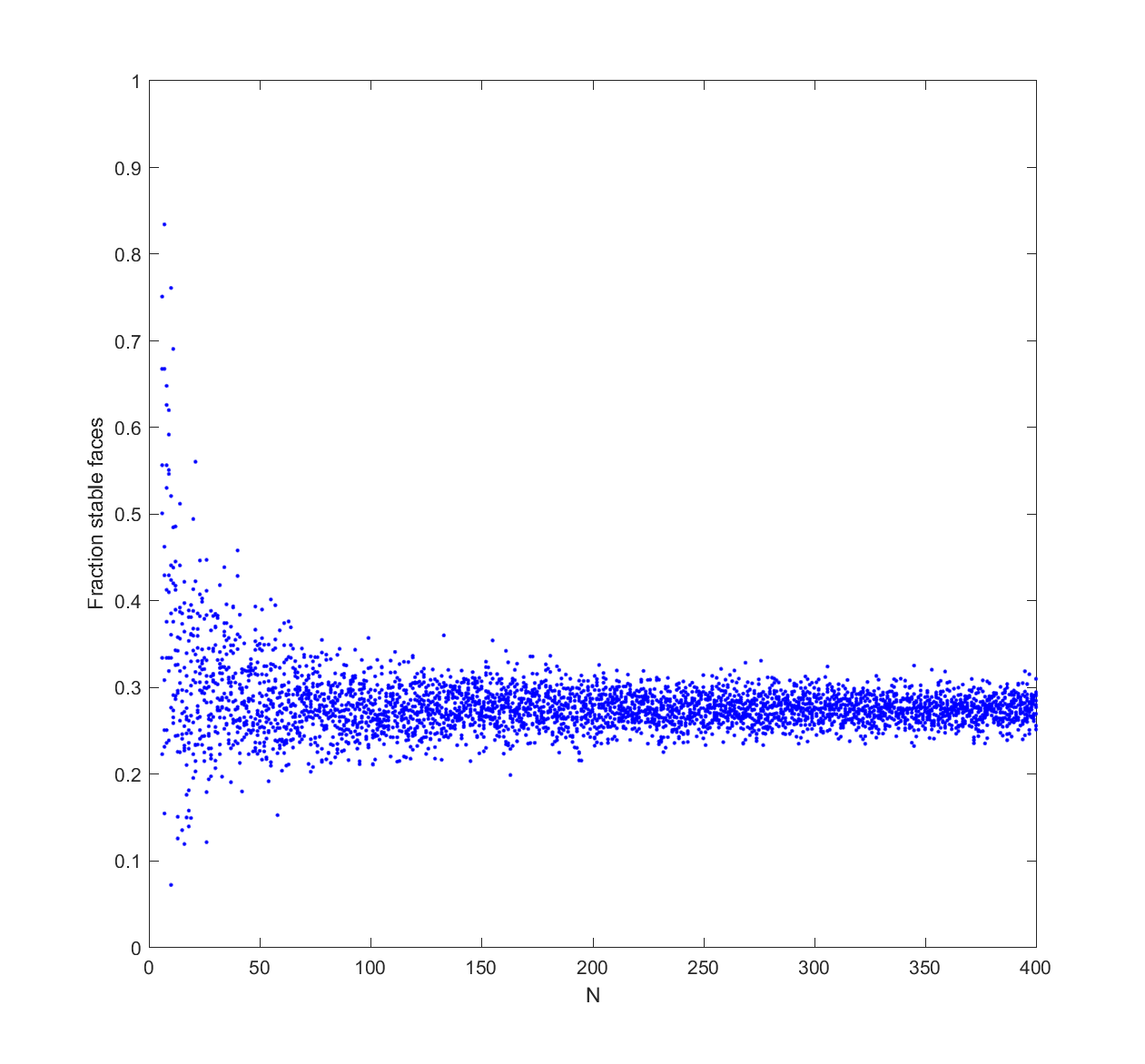
So, what is the average fraction of stable faces on a 3D polyhedron?
Fraction stable faces on 3D convex hulls of N points on a sphere.
It tends to converge to 50%. Doing this in higher dimensions shows the same kind of convergence, although to lower fractions.
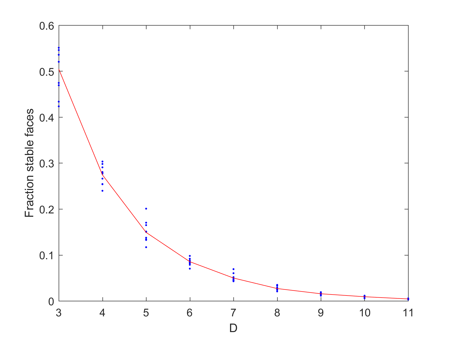
Fraction stable faces on 4D convex hulls of N points on a sphere.Fraction stable faces of N=100 convex hulls in different dimensions. Red line exponential fit.
It looks like the fraction of stable faces declines exponentially with dimensionality.
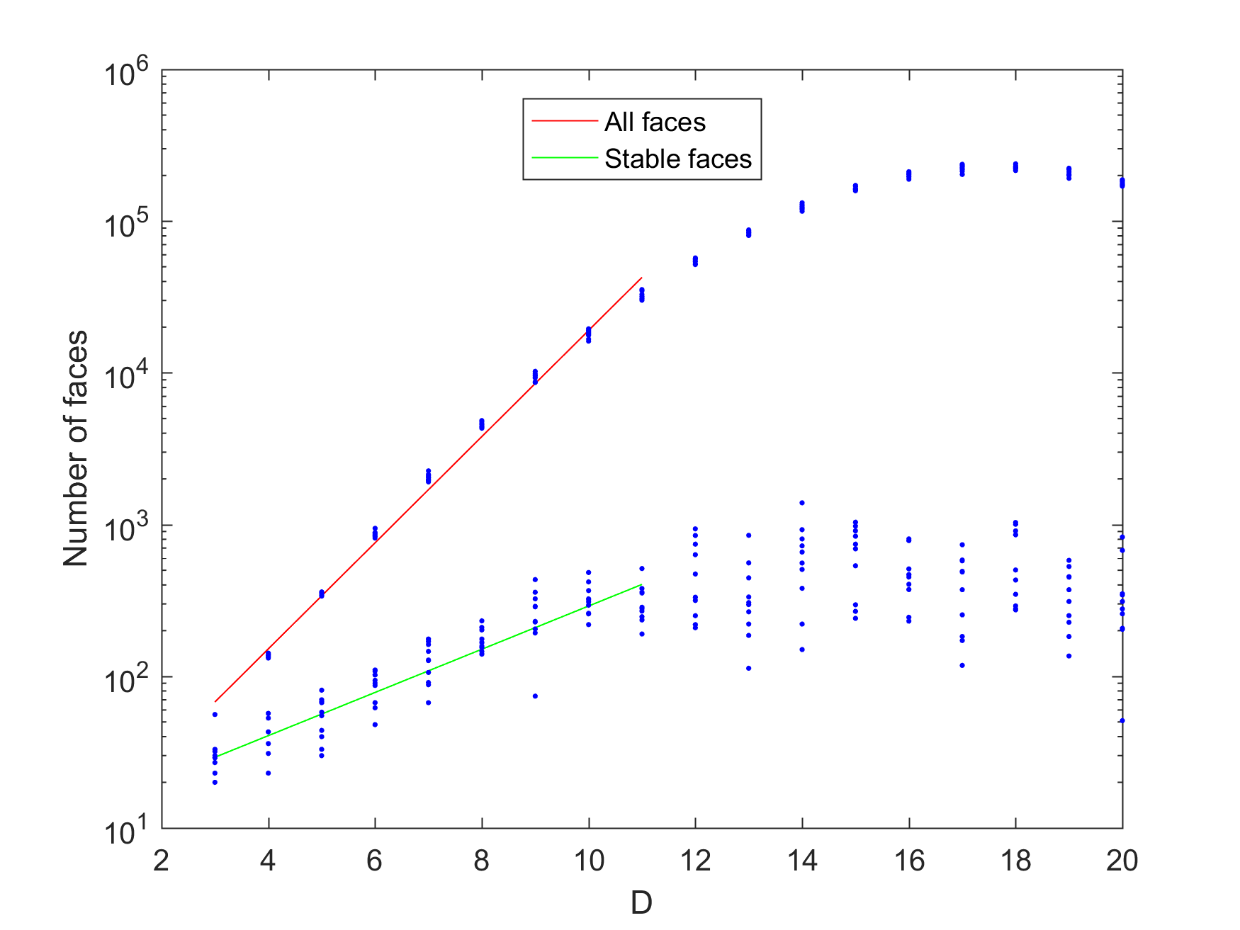
Does this mean that for a sufficiently high dimension it is likely that a random polytope is unistable? The answer is no: the number of faces increases pretty exponentially (as ), but the number of stable faces also increases exponentially with D (as $latex 2^{0.9273 D}$).
Combined plot of number of faces (points with red line) and stable faces (points with green line) as a function of dimension for N=100.
This was based on runs with N=100. Obviously things go much faster if you select a lower N, such as 30. However, as you approach N=D the polytopes become more and more simplex-like, and simplices tend to both have fewer faces and be less stable in high dimensions, so the exponential growth stops. This actually happens far below D; for N=30 the effect is felt already in 11 dimensions. The face growth rates were also lower, with coefficients 1.1621 and 0.4730.
Number of faces and stable faces for N=30 random convex hulls in different dimensions.
(There are some asymptotic formulas known for the growth of the number of faces for random convex hulls; they grow linearly with N but at an accelerating rate with D.)
Stuart Armstrong gave me a very heuristic argument for why there would be so many unstable faces. Consider building up the polytope vertex by vertex, essentially just adding together the simplices from the Delaunay decomposition. If you start from a stable state, eventually you will likely end up with an unstable face. Adding the next vertex will add a simplex to the polyhedron, and the center of mass will move in the direction of the new simplex. To have the face become stable again the shift in center of mass needs to be large enough along the directions parallel to the face to bring the projection back inside the face. But in high dimensional spaces there are many directions you can move in: the probability of a random vector being nearly parallel to another vector is very low. Hence, the next step and the following are likely to preserve the instability. So high dimensional polytopes are likely to have many unstable faces even if they are nicely inscribed in spheres.
The number of steps the polytope rolls over until finding a stable face is also limited: the “drainage basin” of a stable face is a tree, with a branching degree set by D-1 (if faces are D-simplexes). So the number of steps will scale as . Even high-dimensional polytopes will stop flipping quickly in general. (A unistable polytope on the other hand can run through at least half of its faces, so there are some very slow ones too).
The expected minimum distance between two points on this kind of random polytope scales as (if they were optimally distributed it would be ). At the same time, if N is relatively small compared to D (the polytope is simplex-like), the average diameter (the longest edge) of each face seems to approach . Why? I think this is because , the mean of a flipped k=2 Weibull distribution that shows up because of extreme value theory. Meanwhile the average and median cord length between random points on hyperspheres tends towards . Faces hence tends to be fairly wide unless N is large compared to D, but there will typically always be a few very narrow ones that are tricky to balance on.
Stacking no-slip polytopes
What about stacking polytopes?
If you put a polytope on top of another one (assuming no slipping) at first it seems you need to use a stable face of the top polytope, but this is not enough nor necessary.
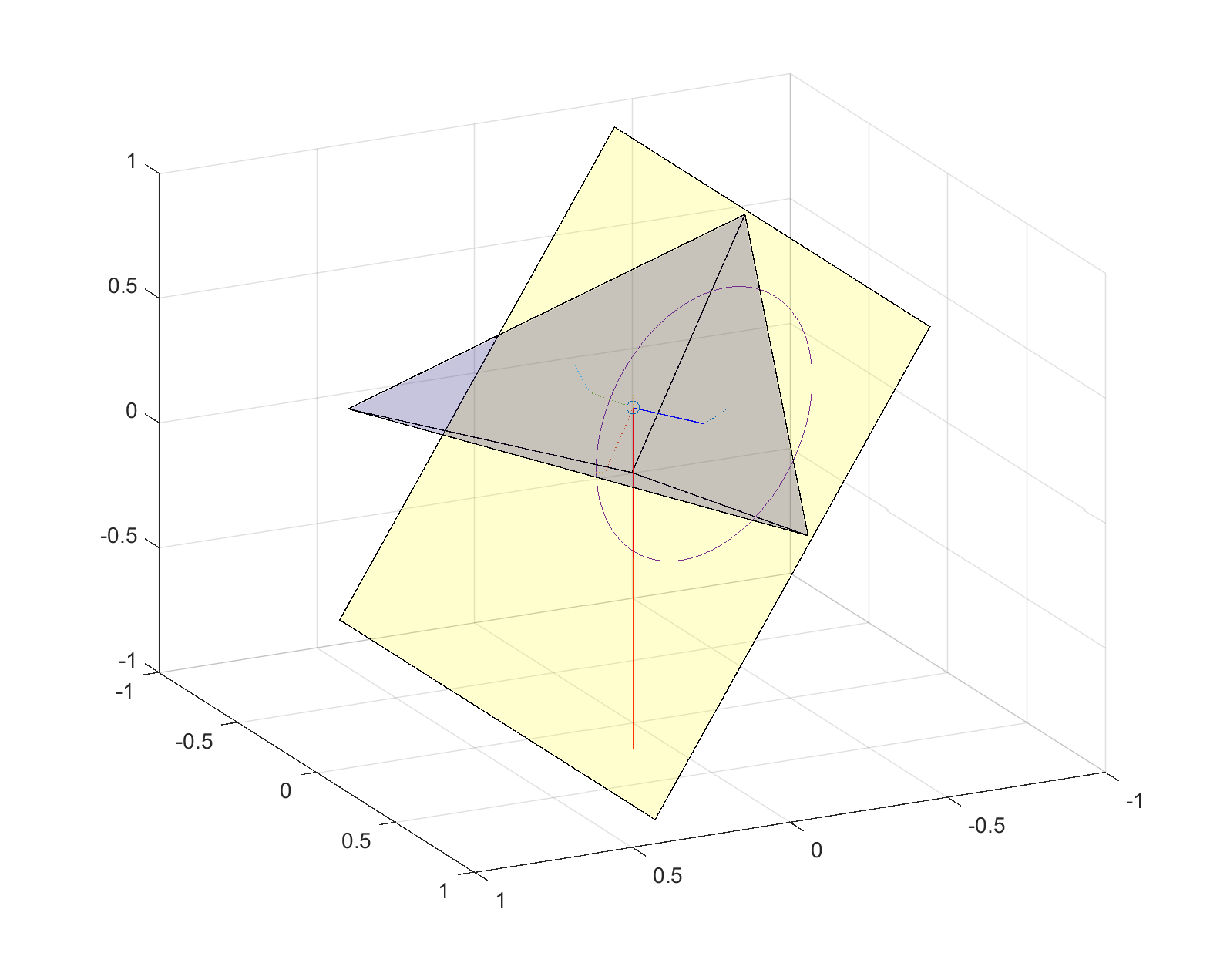
Since the underlying face is likely tilted from the horizontal, the vertical projection of the center of mass has to be within the top face. The upper polytope can be rotated, moving the projection point. The tilt angle (or rather, tilt angles – we are doing this in higher dimensions, remember?) generates a hypersphere of radius around the normal projection point (which is at distance d from the center of mass) where the vertical projection can intersect the face. Only parts of the hypersphere surface that are inside the face represent orientations that are stable. Even an unstable face can (sometimes) be stabilized if you turn it so that the tilted projection is inside, but for sufficiently high angles the hypersphere will be bigger than the face and it cannot be stable.
Stability of polyhedron on tilted surface. The line of gravity from the center of mass intersects the inside the bottom face, so the polyhedron is resting stably. Turning the polyhedron will move the line to some point on the circle, but since all points on the circle are inside the face all orientations are stable.Stability of polyhedron on tilted surface. The line of gravity from the center of mass intersects the outside the bottom face, so the polyhedron is unstable and will flip over. Turning the polyhedron will move the line to some other point on the circle: since some points on the circle are inside the face there are some orientations that are stable.
Having the top polytope stay in place is the first requirement. The second is that the bottom polytope should not become unstable. The new center of mass is moved to a point somewhere along the connecting line between the individual centers of mass of the polytopes, with exact position dependent on their volume ratio (note that turning the top polytope can move the center of mass too). This moves the projection point along the plane of the bottom face, and if it gets outside that face the assembly will tip over.
One can imagine this as adding random (D-1)-dimensional vectors of length 1/N until they reach the edge of the face. I am a bit uncertain about the properties of such random walks (all works on decreasing step size walks I have seen have been in 1D). The harmonic random walk in 1D apparently converges with probability 1, so I think the (D-1)-dimensional one also does it since the distance from the origin to the walker will be smaller than if the walker just kept to a 1D line. Since the expected distance traversed in 1D is $latex E[|X|] \approx 1.0761$ this is actually not a very extreme shift. Given the surprisingly large diameters of the faces if the first condition might be tougher to meet than the second, but this is just a guess.
The no slipping constraint is important. If the polytopes are frictionless, then any transverse force will move them. Hence only polytopes that have some parallel top and bottom stable faces can be stacked, and the problem becomes simpler. There are still surprises there, though: even stacks of rectangular blocks can do surprising things. The block stacking problem also demonstrates that one can have 1/N overhangs (counting downwards), enabling arbitrarily large total overhangs without tipping over. With polytopes with shapes that act as counterweights the overhangs can be even larger.
Uriel’s stacking problems
This leads to what we might call “Uriel’s stacking problem”: given a collection of no-slip convex D-dimensional polytopes, what is the tallest tower that can be constructed from them?
I suspect that this problem is NP-hard. It sounds very much like a knapsack problem, but there is a dependency on previous steps when you add a new polytope that seem to make it harder. It seems that it would not be too difficult to fool a greedy algorithm just trying to put the next polytope on the most topmost face into adding one that makes subsequent steps too unstable, forcing backtracking.
Another related problem: if the polytopes are random convex hulls of N points, what is the distribution of maximum tower heights? What if we just try random stacking?
And finally, what is the maximum overhang that can be done by stacking polytopes from a given set?
As a side effect of a chat about dynamical systems models of metabolic syndrome, I came up with the following nice little toy model showing two kinds of instability: instability because of insufficient dampening, and instability because of too slow dampening.
Where is a N-dimensional vector, A is a matrix with Gaussian random numbers, and constants. The last term should strictly speaking be written as but I am lazy.
The first term causes chaos, as we will see below. The 1/N factor is just to compensate for the N terms. The middle term represents dampening trying to force the system to the origin, but acting with a delay . The final term keeps the dynamics bounded: as becomes large this term will dominate and bring back the trajectory to the vicinity of the origin. However, it is a soft spring that has little effect close to the origin.
Chaos
Let us consider the obvious fixed point . Is it stable? If we calculate the Jacobian matrix there it becomes . First, consider the case where . The eigenvalues of J will be the ones of a random Gaussian matrix with no symmetry conditions. If it had been symmetric, then Wigner’s semicircle rule implies that they would tend to be distributed as as . However, it turns out that this is true for the non-symmetric Gaussian case too. (and might be true for any i.i.d. random numbers). This means that about half of them will have a positive real part, and that implies that the fixed point is unstable: for the system will be orbiting the origin in some fashion, and generically this means a chaotic attractor.
Stability
If grows the diagonal elements of J will become more and more negative. If they are really negative then we essentially have a matrix with a negative diagonal and some tiny off-diagonal terms: the eigenvalues will almost be the diagonal ones, and they are all negative. The origin is a stable attractive fixed point in this limit.
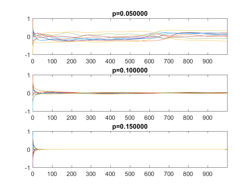
Distribution of real part of the eigenvalues of J=A-pI as the restoring forcing becomes stronger. At p=0.1 all eigenvalues have negative real part.
In between, if we plot the eigenvalues as a function of , we see that the semicircle just linearly moves towards the negative side and when all of it passes over, we shift from the chaotic dynamics to the fixed point. Exactly when this happens depends on the particular A we are looking at and its largest eigenvalue (which is distributed as the Tracy-Widom distribution), but it is generally pretty sharp for large N.
Plots of some x_i over time depending on p. The delay is=1. The top case is chaotic, the middle case is at the crossover point where the eigenvalues become negative, and the lower is beyond it.
Delay
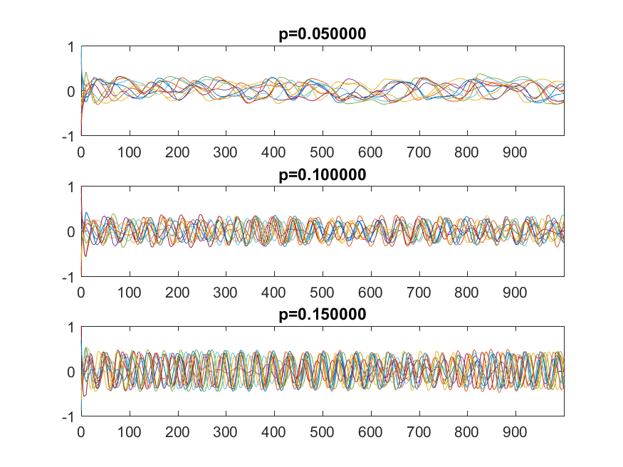
Plots of x over time depending on p, for delay=100. The top case is chaotic, becoming increasingly periodic as p increases.
But what if becomes large? In this case the force moving the trajectory towards the origin will no longer be based on where it is right now, but on where it was seconds earlier. If is small, then this is just minor noise/bias (and the dynamics is chaotic anyway). If it is large, then the trajectory will be pushed in some essentially random direction: we get instability again.
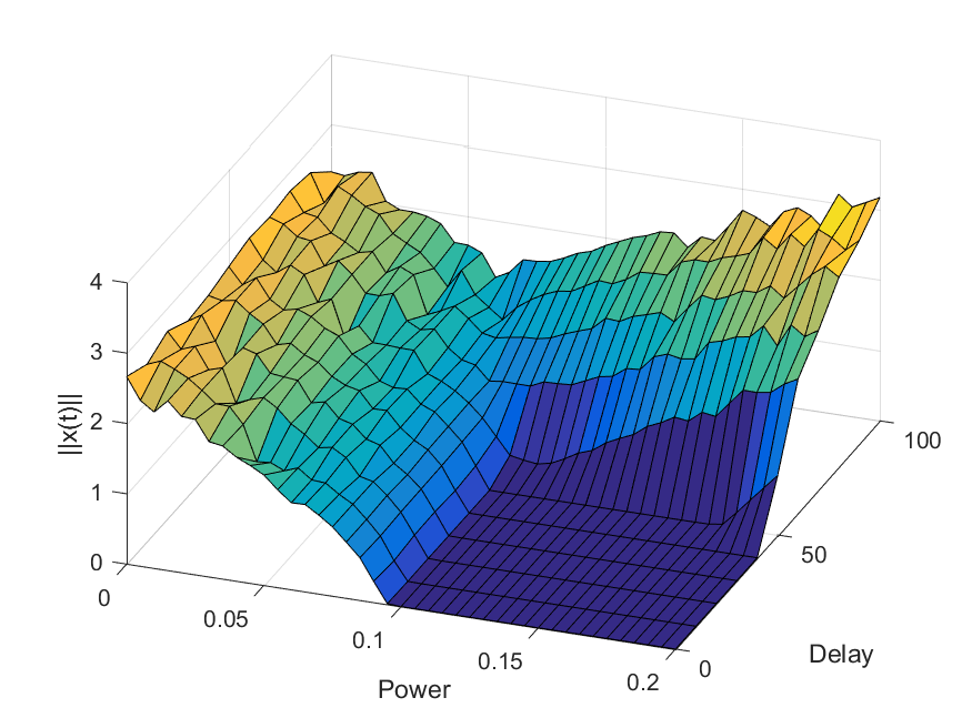
Plot of the average norm |x(t)| for some late value of t as a function of the power and delay. The dark blue square is convergence to zero, the left curved surface is chaotic motion, and the right/back surface is the delay-driven oscillations.
A (very slightly) more stringent way of thinking of it is to plug in into the equation. To simplify, let’s throw away the cubic term since we want to look at behavior close to zero, and let’s use a coordinate system where the matrix is a diagonal matrix . Then for we get , that is, the origin is a fixed point that repels or attracts trajectories depending on its eigenvalues (and we know from above that we can be pretty confident some are positive, so it is unstable overall). For we get . Taylor expansion to the first order and rearranging gives us . The numerator means that as grows, each eigenvalue will eventually get a negative real part: that particular direction of dynamics becomes stable and attracted to the origin. But the denominator can sabotage this: it gets large enough it can move the eigenvalue anywhere, causing instability.
So there you are: if you try to keep a system stable, make sure the force used is up to the task so the inherent recalcitrance cannot overwhelm it, and make sure the direction actually corresponds to the current state of the system.
Playing with Matlab, I plotted the location of the zeros of a polynomial with normally distributed coefficients in the complex plane. It was nearly a circle:
Zeros of a 100-degree polynomial with normally distributed random coefficients.
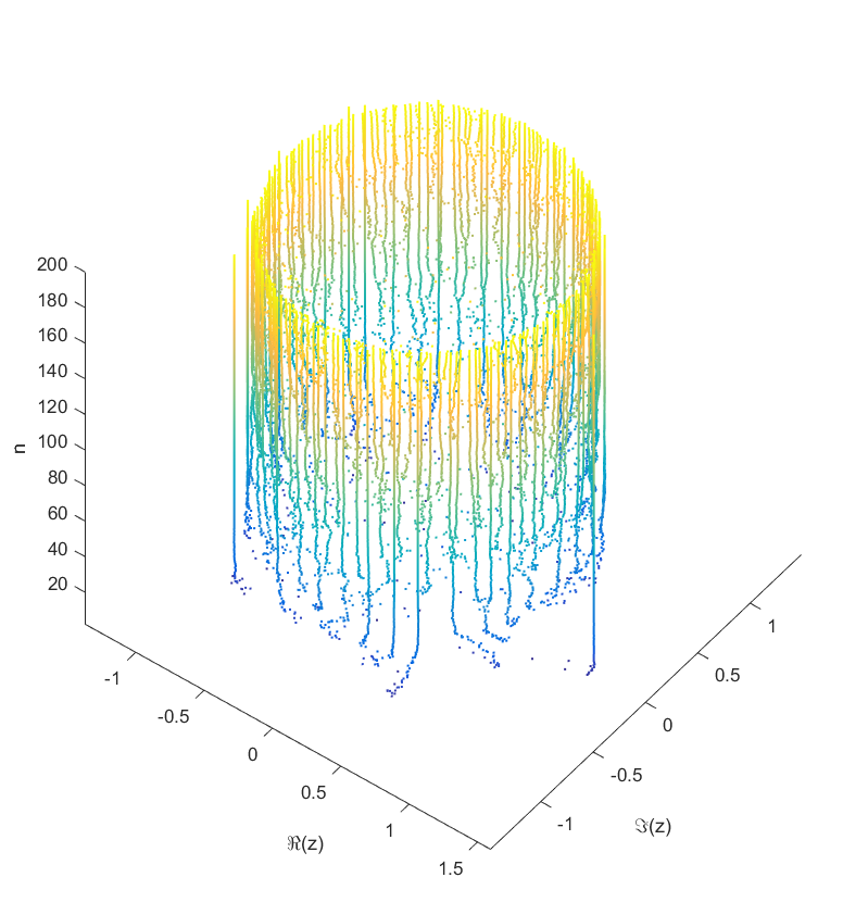
Locations of the zeros of a polynomial with a given sequence of normally distributed coefficients, as a function of degree.
As you add more and more terms to the polynomial the zeros approach the unit circle. Each new term perturbs them a bit: at first they move around a lot as the degree goes up, but they soon stabilize into robust positions (“young” zeros move more than “old” zeros). This seems to be true regardless of whether the coefficients set in “little-endian” or “big-endian” fashion.
But then I decided to move things around: what if the coefficient on the leading term changed? How would the zeros move? I looked at the polynomial where were from some suitable random sequence and could run around . Since the leading coefficient would start and end up back at 1, I knew all zeros would return to their starting position. But in between, would they jump around discontinuously or follow orderly paths?
Continuity is actually guaranteed, as shown by (Harris & Martin 1987). As you change the coefficients continuously, the zeros vary continuously too. In fact, for polynomials without multiple zeros, the zeros vary analytically with the coefficients.
As runs from 0 to the roots move along different orbits. Some end up permuted with each other.
Movement of the zeros of polynomials with random coefficients as the leading coefficient traverses the unit circle. Colour denotes phase, zeros marked by squares.
For low degrees, most zeros participate in a large cycle. Then more and more zeros emerge inside the unit circle and stay mostly fixed as the polynomial changes. As the degree increases they congregate towards the unit circle, while at least one large cycle wraps most of them, often making snaking detours into the zeros near the unit circle and then broad bows outside it.
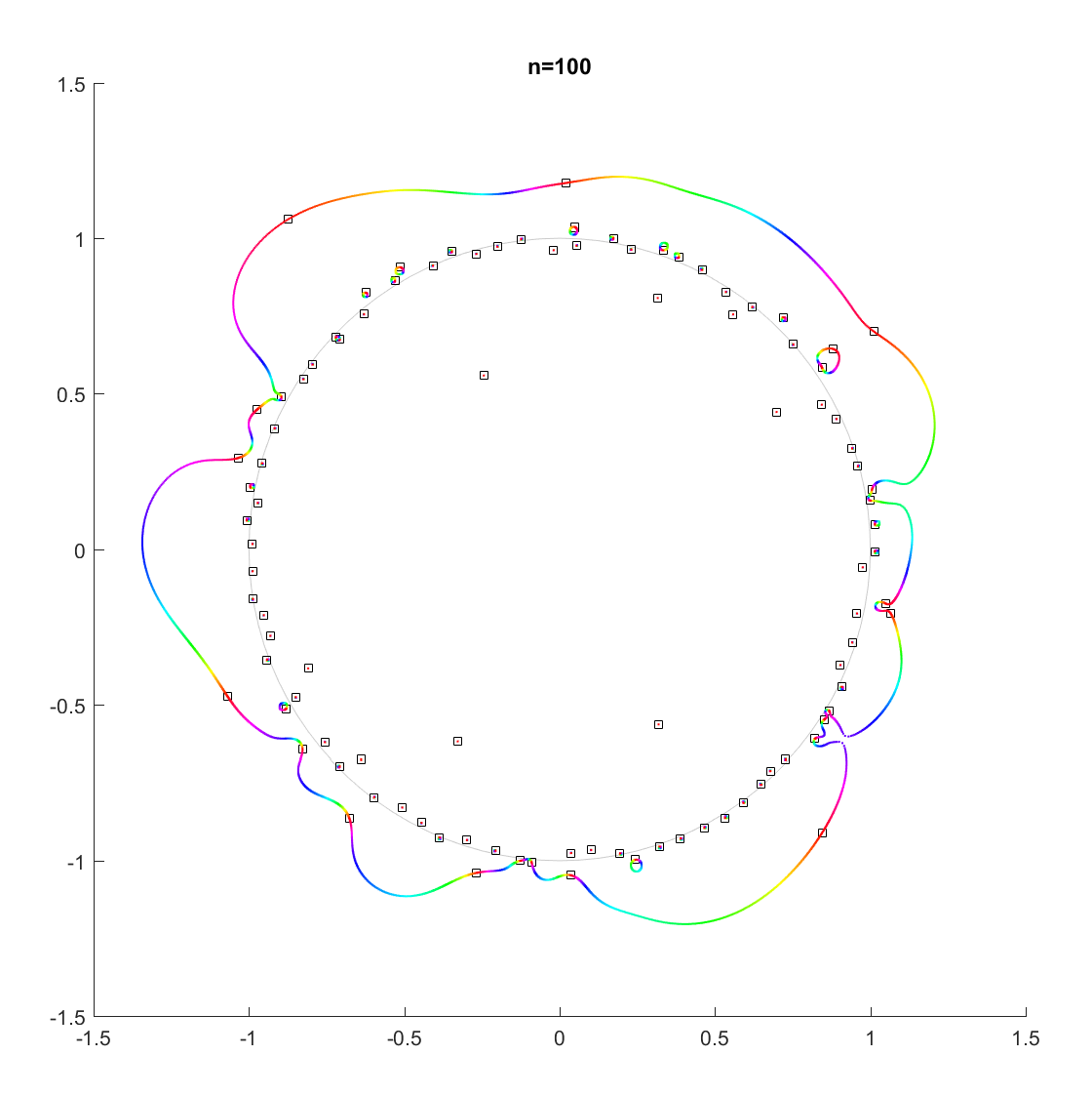
Movement of the zeros of a random degree 100 polynomial.
In the above example, there is a 21-cycle, as well as a 2-cycle around 2 o’clock. The other zeros stay mostly put.
The real question is what determines the cycles? To understand that, we need to change not just the argument but the magnitude of .
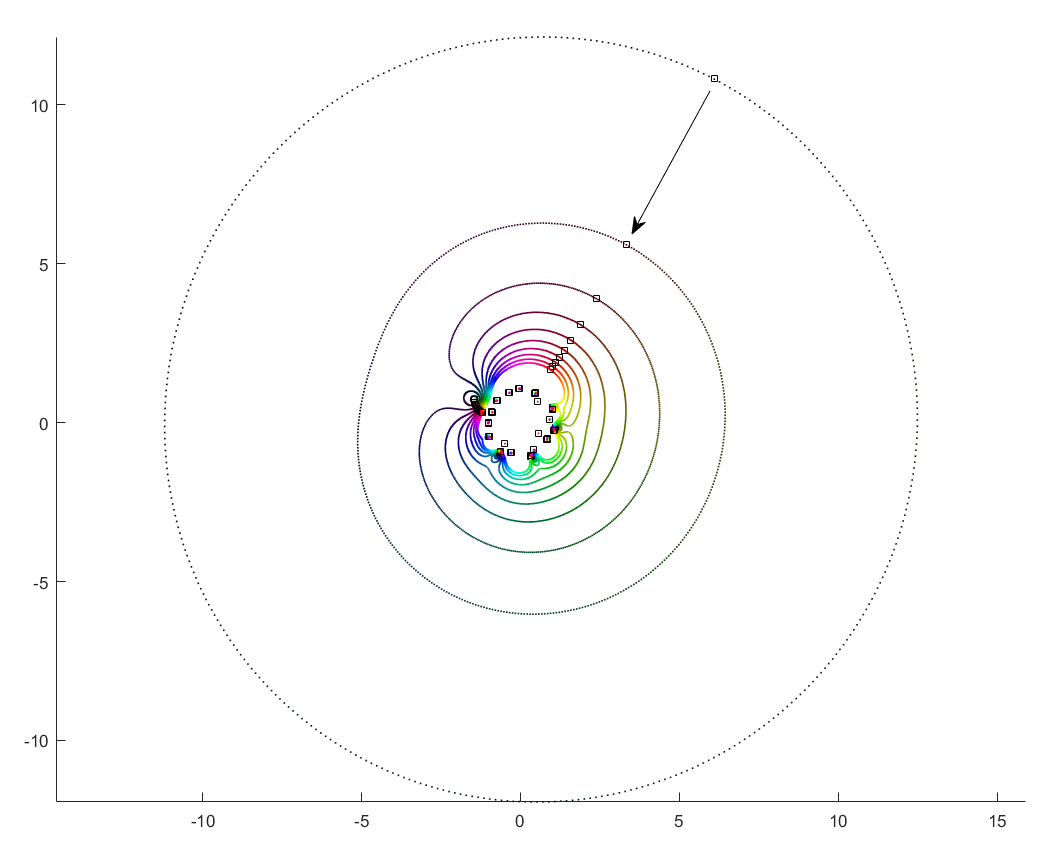
Orbits of roots as the magnitude of the leading coefficient increases from zero to one.
What happens if we slowly increase the magnitude of the leading term, letting for a r that increases from zero? It turns out that a new zero of the function zooms in from infinity towards the unit circle. A way of seeing this is to look at the polynomial as : the second term is nonzero and large in most places, so if is small the factor must be large (and opposite) to outweigh it and cause a zero. The exception is of course close to the zeros of , where the perturbation just moves them a tiny bit: there is a counterpart for each of the zeros of among the zeros of . While the new root is approaching from outside, if we play with it will make a turn around the other zeros: it is alone in its orbit, which also encapsulates all the other zeros. Eventually it will start interacting with them, though.
Orbits of roots as the magnitude of the leading coefficient decreases from 100 to one.
If you instead start out with a large leading term, , then the polynomial is essentially and the zeros the n-th roots of . All zeros belong to the same roughly circular orbit, moving together as makes a rotation. But as decreases the shared orbit develops bulges and dents, and some zeros pinch off from it into their own small circles. When does the pinching off happen? That corresponds to when two zeros coincide during the orbit: one continues on the big orbit, the other one settles down to be local. This is the one case where the analyticity of how they move depending on breaks down. They still move continuously, but there is a sharp turn in their movement direction. Eventually we end up in the small term case, with a single zero on a large radius orbit as .
This pinching off scenario also suggests why it is rare to find shared orbits in general: they occur if two zeros coincide but with others in between them (e.g. if we number them along the orbit, , with to separate). That requires a large pinch in the orbit, but since it is overall pretty convex and circle-like this is unlikely.
Allowing to run from to 0 and over would cover the entire complex plane (except maybe the origin): for each z, there is some where . This is fairly obviously . This function has a central pole, surrounded by zeros corresponding to the zeros of . The orbits we have drawn above correspond to level sets , and the pinching off to saddle points of this surface. To get a multi-zero orbit several zeros need to be close together enough to cause a broad valley.
Graph of the log-magnitude of f(z), the function mapping a point in the plane to the value of [latex]c_n[/latex] that causes a zero to appear there for [latex]P_n(z)[/latex].
There you have it, a rough theory of dancing zeros.
If there are key ideas needed to produce some important goal (like AI), there is a constant probability per researcher-year to come up with an idea, and the researcher works for years, what is the the probability of success? And how does it change if we add more researchers to the team?
The most obvious approach is to think of this as y Bernouilli trials with probability p of success, quickly concluding that the number of successes n at the end of y years will be distributed as . Unfortunately, then the actual answer to the question will be which is a real mess…
A somewhat cleaner way of thinking of the problem is to go into continuous time, treating it as a homogeneous Poisson process. There is a rate of good ideas arriving to a researcher, but they can happen at any time. The time between two ideas will be exponentially distributed with parameter . So the time until a researcher has ideas will be the sum of exponentials, which is a random variable distributed as the Erlang distribution: .
Just like for the discrete case one can make a crude argument that we are likely to succeed if is bigger than the mean (or ) we will have a good chance of reaching the goal. Unfortunately the variance scales as – if the problems are hard, there is a significant risk of being unlucky for a long time. We have to consider the entire distribution.
Unfortunately the cumulative density function in this case is which is again not very nice for algebraic manipulation. Still, we can plot it easily.
Before we do that, let us add extra researchers. If there are researchers, equally good, contributing to the idea generation, what is the new rate of ideas per year? Since we have assumed independence and a Poisson process, it just multiplies the rate by a factor of . So we replace with everywhere and get the desired answer.
This is a plot of the case .
What we see is that for each number of scientists it is a sigmoid curve: if the discovery probability is too low, there is hardly any chance of success, when it becomes comparable to it rises, and sufficiently above we can be almost certain the project will succeed (the yellow plateau). Conversely, adding extra researchers has decreasing marginal returns when approaching the plateau: they make an already almost certain project even more certain. But they do have increasing marginal returns close to the dark blue “floor”: here the chances of success are small, but extra minds increase them a lot.
We can for example plot the ratio of success probability for to the one researcher case as we add researchers:
Even with 10 researchers the success probability is just 40%, but clearly the benefit of adding extra researchers is positive. The curve is not quite exponential; it slackens off and will eventually become a big sigmoid. But the overall lesson seems to hold: if the project is a longshot, adding extra brains makes it roughly exponentially more likely to succeed.
It is also worth recognizing that in this model time is on par with discovery rate and number of researchers: what matters is the product and how it compares to .
This all assumes that ideas arrive independently, and that there are no overheads for having a large team. In reality these things are far more complex. For example, sometimes you need to have idea 1 or 2 before idea 3 becomes possible: that makes the time of that idea distributed as an exponential plus the distribution of . If the first two ideas are independent and exponential with rates , then the minimum is distributed as an exponential with rate . If they instead require each other, we get a non-exponential distribution (the pdf is ). Some discoveries or bureaucratic scalings may change the rates. One can construct complex trees of intellectual pathways, unfortunately quickly making the distributions impossible to write out (but still easy to run Monte Carlo on). However, as long as the probabilities and the induced correlations small, I think we can linearise and keep the overall guess that extra minds are exponentially better.
In short: if the cooks are unlikely to succeed at making the broth, adding more is a good idea. If they already have a good chance, consider managing them better.
While surfing the web I came across a neat Julia set, defined by iterating for some complex constant c. Here are some typical pictures, and two animations: one moving around a circle in the c-plane, one moving slowly down from c=1 to c=0.
The points behind the set
What is going on?
The first step in analysing fractals like this is to find the fixed points and their preimages. is clearly mapped to itself. The term will tend to make large magnitude iterates approach infinity, so it is an attractive fixed point.
is a preimage of infinity: iterates falling on zero will be mapped onto infinity. Nearby points will also end up attracted to infinity, so we have a basin of attraction to infinity around the origin. Preimages of the origin will be mapped to infinity in two steps: has the solutions – this is where the pentagonal symmetry comes from, since these five points are symmetric. Their preimages and so on will also be mapped to infinity, so we have a hierarchy of basins of attraction sending points away forming some gasket-like structure. The Julia set consists of the points that never gets mapped away, the boundary of this hierarchy of basins.
The other fixed points are defined by , which can be rearranged into . They don’t have any neat expression and actually do not affect the big picture dynamics as much. The main reason seems to be that they are unstable. However, their location and the derivative close to them affect the shapes in the Julia set as we will see. Their preimages will be surrounded by the same structures (scaled and rotated) as they have.
Below are examples with preimages of zero marked as white circles, fixed points as red crosses, and critical points as black squares.
The set behind the points
A simple way of mapping the dynamics is to look at the (generalized) Mandelbrot set for the function, taking a suitable starting point and mapping out its fate in the c-plane. Why that particular point? Because it is one of the critical point where , and a theorem by Julia and Fatou tells us that its fate indicates whether the Julia set is filled or dust-like: bounded orbits of the critical points of a map imply a connected Julia set. When c is in the Mandelbrot set the Julia image has “thick” regions with finite area that do not escape to infinity. When c is outside, then most points end up at infinity, and what remains is either dust or a thin gasket with no area.
The set is much smaller than the vanilla Mandelbrot, with a cuspy main body surrounded by a net reminiscent of the gaskets in the Julia set. It also has satellite vanilla Mandelbrots, which is not surprising at all: the square term tends to dominate in many locations. As one zooms into the region near the origin a long spar covered in Mandelbrot sets runs towards the origin, surrounded by lacework.
One surprising thing is that the spar does not reach the origin – it stops at . Looking at the dynamics, above this point the iterates of the critical point jump around in the interval [0,1], forming a typical Feigenbaum cascade of period doubling as you go out along the spar (just like on the spar of the vanilla Mandelbrot set). But at this location points now are mapped outside the interval, running off to infinity: one of the critical points breaches a basin boundary, causing iterates to run off and the earlier separate basins to merge. Below this point the dynamics is almost completely dominated by the squaring, turning the Julia set into a product of a Cantor set and a circle (a bit wobbly for higher c; it is all very similar to KAM torii). The empty spaces correspond to the regions where preimages of zero throw points to infinity, while along the wobbly circles points get their argument angles multiplied by two for every iteration by the dominant quadratic term: they are basically shift maps. For c=0 it is just the filled unit disk.
So when we allow c to move around a circle as in the animations, the part that passes through the Mandelbrot set has thick regions that thin as we approach the edge of the set. Since the edge is highly convoluted the passage can be quite complex (especially if the circle is “tangent” to it) and the regions undergo complex twisting and implosions/explosions. During the rest of the orbit the preimages just quietly rotate, forming a fractal gasket. A gasket that sometimes looks like a model of the hyperbolic plane, since each preimage has five other preimages, naturally forming an exponential hierarchy that has to be squeezed into a finite roughly circular space.
I was not first with this idea. In fact, F.F. de Brito used this back in 1992 to demonstrate that there exist complete embedded minimal surfaces in 3-space that are contained between two planes.
Here is the surface defined by the function , the Taylor series that only includes all prime powers, combined with .
Close to zero, the surface is flat. Away from zero it begins to wobble as increasingly high powers in the series begin to dominate. It behaves very much like a higher-degree Enneper surface, but with a wobble that is composed of smaller wobbles. It is cool to consider that this apparently irregular pattern corresponds to the apparently irregular pattern of all primes.
Recently I chatted with a mathematician friend about generating functions in combinatorics. Normally they are treated as a neat symbolic trick: you have a sequence (typically how many there are of some kind of object of size ), you formally define a function , you derive some constraints on the function, and from this you get a formula for the or other useful data. Convergence does not matter, since this is purely symbolic. We used this in our paper counting tie knots. It is a delightful way of solving recurrence relations or bundle up moments of probability distributions.
I innocently wondered if the function (especially its zeroes and poles) held any interesting information. My friend told me that there was analytic combinatorics: you can actually take seriously as a (complex) function and use the powerful machinery of complex analysis to calculate asymptotic behavior for the from the location and type of the “dominant” singularities. He pointed me at the excellent course notes from a course at Princeton linked to the textbook by Philippe Flajolet and Robert Sedgewick. They show a procedure for taking combinatorial objects, converting them symbolically into generating functions, and then get their asymptotic behavior from the properties of the functions. This is extraordinarily neat, both in terms of efficiency and in linking different branches of math.
Plot of z/(1-z-z^2), the generating function of the Fibonacci numbers. It has poles at (1+sqrt(5))/2 (the dominant pole giving the overall asymptotic growth of Fibonacci numbers) and (1-sqrt(5))/2, which does not contribute much to the asymptotic behavior.
In our case, one can show nearly by inspection that the number of Fink-Mao tie knots grow with the number of moves as , while single tuck tie knots grow as .
Analytic functions behaving badly
The second piece of math I found this weekend was about random Taylor series and lacunary functions.
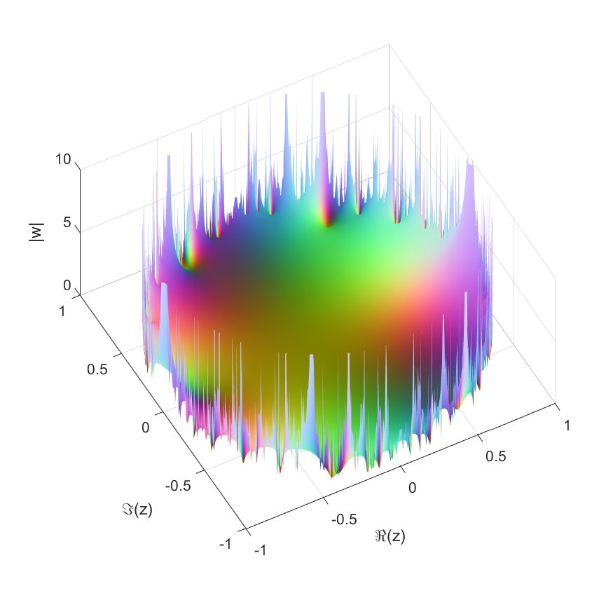
If where are independent random numbers, what kind of functions do we get? Trying it with complex Gaussian produces a disk of convergence with some nondescript function on the inside.
Plot of function with a Gaussian Taylor series. Color corresponds to stereographic mapping of the complex plane to a sphere, with infinity being white and zeros black. The domain of convergence is the unit circle.
Replacing the complex Gaussian with a real one, or uniform random numbers, or even power-law numbers gives the same behavior. They all seem to have radius 1. This is not just a vanilla disk of convergence (where an analytic function reaches a pole or singularity somewhere on the boundary but is otherwise fine and continuable), but a natural boundary – that is, a boundary so dense with poles or singularities that continuation beyond it is not possible at all.
The locus classicus about random Taylor series is apparently Kahane, J.-P. (1985), Some Random Series of Functions. 2nd ed., Cambridge University Press, Cambridge.
A naive handwave argument is that for we have an exponentially decaying sequence of , so if the have some finite average size and not too divergent variance we should expect convergence, while outside the unit circle any nonzero will allow it to diverge. We can even invoke the Markov inequality to argue that a series would converge if converges. However, this is not correct enough for proper mathematics. One entirely possible Gaussian outcome is or worse. We need to speak of probabilistic convergence.
Andrés E. Caicedo has a good post about how to approach it properly. The “trick” is the awesome Kolmogorov zero-one law that implies that since the radius of convergence depends on the entire series X_n rather than any finite subset (and they are all independent) it will be a constant.
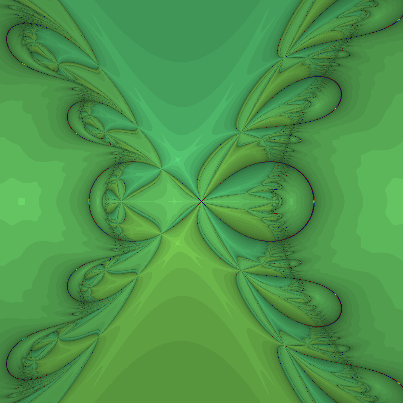
This kind of natural boundary disk of convergence may look odd to beginning students of complex analysis: after all, none of the functions we normally encounter behave like this. Except that this is of course selection bias. If you look at the example series for lacunary functions they all look like fairly reasonable sparse Taylor series like $z+z^4+z^8+z^16+^32+\lddots$. In calculus we are used to worrying that the coefficients in front of the z-terms of a series don’t diminish fast enough: having fewer nonzero terms seems entirely innocuous. But as Hadamard showed, it is enough that the size of the gaps grow geometrically for the function to get a natural boundary (in fact, even denser series do this – for example having just prime powers). The same is true for Fourier series. Weierstrass’ famous continuous but nowhere differentiable function is lacunary (in his 1880 paper on analytic continuation he gives the example of an uncontinuable function). In fact, as Emile Borel found and Steinhardt eventually proved in a stricter sense, in general (“almost surely”) a Taylor series isn’t continuable because of boundaries.
The function [latex]sum_p z^p[/latex], where [latex]p[/latex] runs over the primes.
One could of course try to combine the analytic combinatorics with the lacunary stuff. In a sense a lacunary generating function is a worst case scenario for the singularity-measuring methods used in analytical combinatorics since you get an infinite number of them at a finite and equal distance, and now have to average them together somehow. Intuitively this case seems to correspond to counting something that becomes rarer at a geometric rate or faster. But the Borel-Steinhardt results suggest that even objects that do not become rare could have nasty natural boundaries – if the number were due to something close enough to random we should expect estimating asymptotics to be hard. The funniest example I can think of is the number of roots of Chaitin-style Diophantine equations where for each it is an independent arithmetic fact whether there are any: this is hardcore random, and presumably the exact asymptotic growth rate will be uncomputable both practically and theoretically.

![[\tanh(x),\tanh(y)]](https://s0.wp.com/latex.php?latex=%5B%5Ctanh%28x%29%2C%5Ctanh%28y%29%5D&bg=ffffff&fg=000000&s=0 "[\tanh(x),\tanh(y)]")
![[-1,1]\times [-1,1]](https://s0.wp.com/latex.php?latex=%5B-1%2C1%5D%5Ctimes+%5B-1%2C1%5D&bg=ffffff&fg=000000&s=0 "[-1,1]\times [-1,1]")
![(1/2)+(1/2)[\tanh(|z-1|-1), \tanh(|z+1|-1), \tanh(|z-i|-1)]](https://s0.wp.com/latex.php?latex=%281%2F2%29%2B%281%2F2%29%5B%5Ctanh%28%7Cz-1%7C-1%29%2C+%5Ctanh%28%7Cz%2B1%7C-1%29%2C+%5Ctanh%28%7Cz-i%7C-1%29%5D&bg=ffffff&fg=000000&s=0 "(1/2)+(1/2)[\tanh(|z-1|-1), \tanh(|z+1|-1), \tanh(|z-i|-1)]")


") the zeros will typically form a curve in the plane. In order to get discrete zeros we typically need to have two functions to produce a zero set. We can think of it as a map from R2 to R2
the zeros will typically form a curve in the plane. In order to get discrete zeros we typically need to have two functions to produce a zero set. We can think of it as a map from R2 to R2 ![F(x)=[f_1(x_1,x_2), f_2(x_1,x_2)]](https://s0.wp.com/latex.php?latex=F%28x%29%3D%5Bf_1%28x_1%2Cx_2%29%2C+f_2%28x_1%2Cx_2%29%5D+&bg=ffffff&fg=000000&s=0 "F(x)=[f_1(x_1,x_2), f_2(x_1,x_2)]") where the x’es are 2D vectors. In this case Newton’s method turns into solving the linear equation system
where the x’es are 2D vectors. In this case Newton’s method turns into solving the linear equation system (x_{n+1}-x_n)=-F(x_n)") where
where ") is the Jacobian matrix (
is the Jacobian matrix ( ) and
) and  now denotes the n’th iterate.
![F=[x^3-x-y, y^3-x-y]](https://s0.wp.com/latex.php?latex=F%3D%5Bx%5E3-x-y%2C+y%5E3-x-y%5D&bg=ffffff&fg=000000&s=0 "F=[x^3-x-y, y^3-x-y]") . Below is a plot of the first and second components (red and green), as well as a blue plane for zero values. The zeros of the function are the three points where red, green and blue meet.
. Below is a plot of the first and second components (red and green), as well as a blue plane for zero values. The zeros of the function are the three points where red, green and blue meet. , one at
  , and one at
  The middle one has a region of troublesomely similar function values – the red and green surfaces are tangent there.
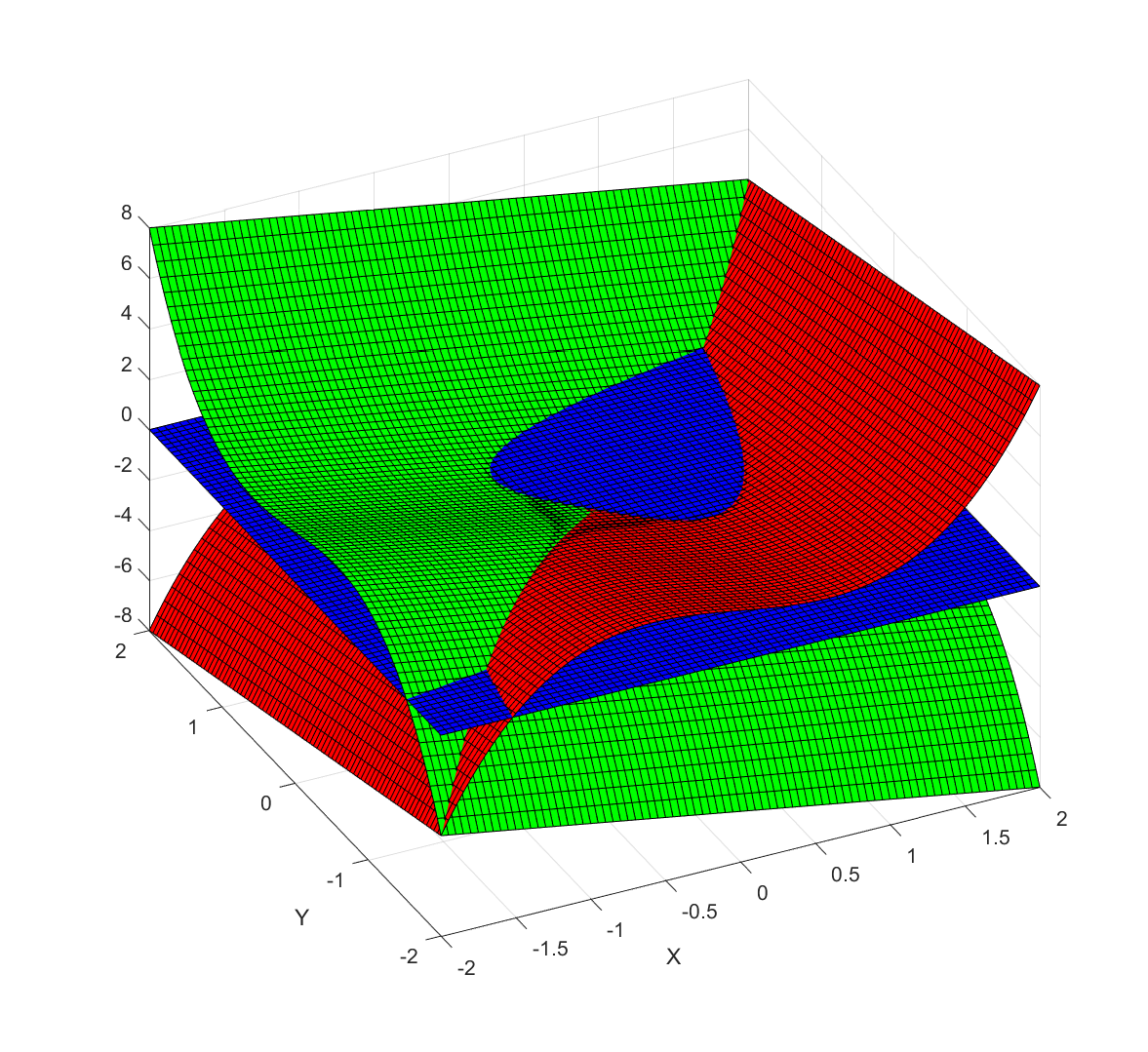
![Behavior of Newton's method in 2D for F=[x^3-x-y, y^3-x-y]. Color denotes value of x+y, with darkening for slow convergence.](http://aleph.se/andart2/wp-content/uploads/2016/12/newton2dp1.png)
 (where
  and
and  if the matrix has the usual
 ![[a b; c d]](https://s0.wp.com/latex.php?latex=%5Ba+b%3B+c+d%5D&bg=ffffff&fg=000000&s=0 "[a b; c d]") form). So if the trace and determinant are randomly chosen, we should expect a majority of cases to be non-rotational.
form). So if the trace and determinant are randomly chosen, we should expect a majority of cases to be non-rotational.![F=[x \cos(\theta) + y \sin(\theta), x\sin(\theta)+y\cos(\theta)]](https://s0.wp.com/latex.php?latex=F%3D%5Bx+%5Ccos%28%5Ctheta%29+%2B+y+%5Csin%28%5Ctheta%29%2C+x%5Csin%28%5Ctheta%29%2By%5Ccos%28%5Ctheta%29%5D&bg=ffffff&fg=000000&s=0 "F=[x \cos(\theta) + y \sin(\theta), x\sin(\theta)+y\cos(\theta)]") . This is of course just a rotation by the angle theta, and it does not have very interesting zeros.
. This is of course just a rotation by the angle theta, and it does not have very interesting zeros. \cos(\theta)")
 \sin(\theta),")
![(x^3-x-y) \sin(\theta)+(y^3-y-x) \cos(\theta) ]](https://s0.wp.com/latex.php?latex=%28x%5E3-x-y%29+%5Csin%28%5Ctheta%29%2B%28y%5E3-y-x%29+%5Ccos%28%5Ctheta%29+%5D&bg=ffffff&fg=000000&s=0 "(x^3-x-y) \sin(\theta)+(y^3-y-x) \cos(\theta) ]") . The result is fun, but still far from baroque:
. The result is fun, but still far from baroque: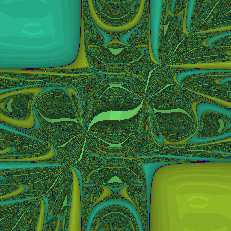
 to make the dynamics even more complex:
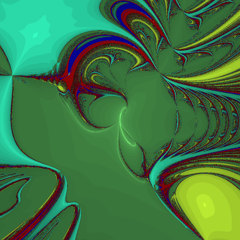
![F=[x^3-3xy^2-1, 3x^2y-y^3]](https://s0.wp.com/latex.php?latex=F%3D%5Bx%5E3-3xy%5E2-1%2C+3x%5E2y-y%5E3%5D&bg=ffffff&fg=000000&s=0 "F=[x^3-3xy^2-1, 3x^2y-y^3]") (which produces the archetypal
(which produces the archetypal =z^3-1") Newton fractal).
Newton fractal).![Newton fractal for F=[x^3-3xy^2-1, 3x^2y-y^3].](http://aleph.se/andart2/wp-content/uploads/2016/12/newtonpert0.png)
![F=[x^3-3xy^2-1 + \epsilon x, 3x^2y-y^3]](https://s0.wp.com/latex.php?latex=F%3D%5Bx%5E3-3xy%5E2-1+%2B+%5Cepsilon+x%2C+3x%5E2y-y%5E3%5D&bg=ffffff&fg=000000&s=0 "F=[x^3-3xy^2-1 + \epsilon x, 3x^2y-y^3]") , then for
, then for  we get:
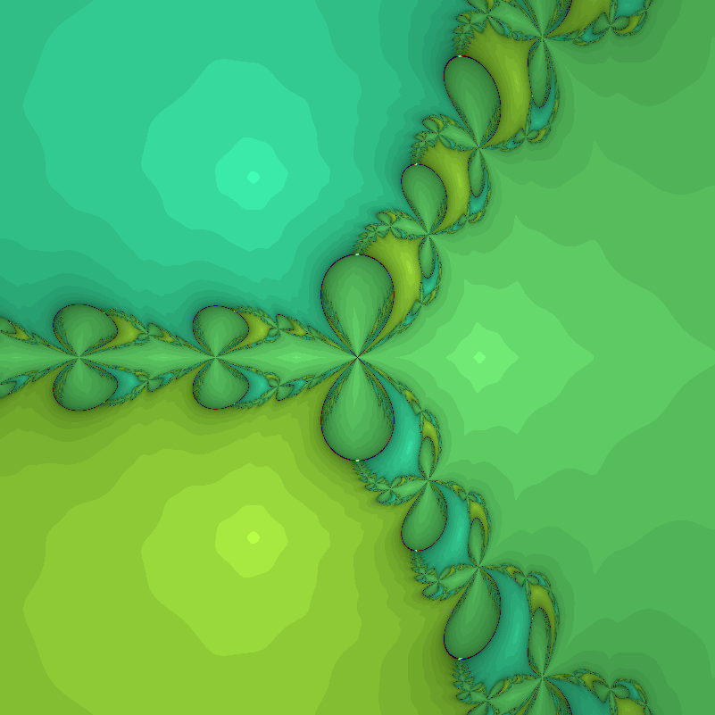
 possible scenarios, one of which (
 ) will come about. They have probability
  . We allocate a unit budget of effort to the scenarios:
  . For the scenario that comes about, we get utility
  (diminishing returns).
 .
.  corresponds to even allocation, 1 proportional to the likelihood, >1 to favoring the most likely scenarios. In the following I will run Monte Carlo simulations where the probabilities are randomly generated each instantiation. The outer bluish envelope represents the 95% of the outcomes, the inner ranges from the lower to the upper quartile of the utility gained, and the red line is the expected utility.
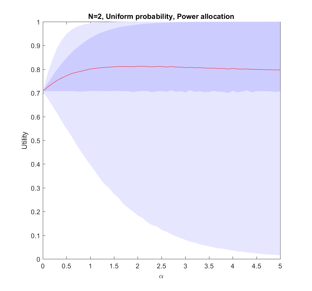
 case: we have two possible scenarios with probability
  and
and  (where
  utility on average, but if we put in more effort on the more likely case we will get up to 0.8 utility. As we focus more and more on the likely case there is a corresponding increase in variance, since we may guess wrong and lose out. But 75% of the time we will do better than if we just allocated evenly. Still, allocating nearly everything to the most likely case means that one does lose out on a bit of hedging, so the expected utility declines slowly for large
  .
.
 case (where the probabilities are allocated based on a flat
  ), but we are not able to allocate perfectly. A more plausible model would give us probability estimates instead of the actual probabilities.
 ). The larger N is, the less likely it is that we focus on the right scenario since we know nothing. The rationality of ignoring irrelevant information is pretty obvious.
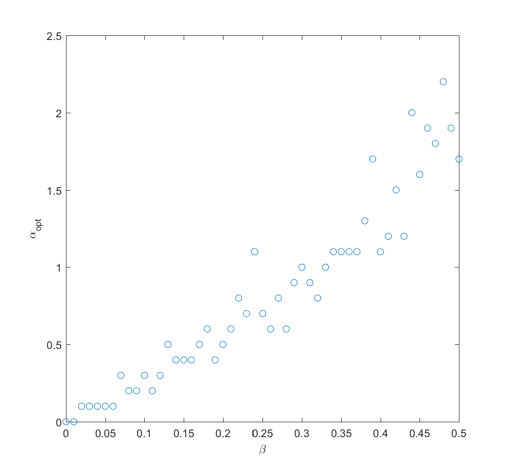
 . In fact, we can mix in just a bit (
 ) of the true probability and get a fairly good guess where to allocate effort (i.e. we allocate effort as
 Q_i)^\alpha") where
where  is uncorrelated noise probabilities). The optimal alpha grows roughly linearly with
  in this case.
 to the different scenarios we get better information about the probabilities, and can now reallocate. A simple model may be that the standard deviation of noise behaves as
  where
where  is the effort placed in exploring the probability of scenario
  . So if we begin by allocating uniformly we will have noise at reallocation of the order of
  . We can set
 =\sqrt{\gamma/N}/C") , where
, where  is some constant denoting how tough it is to get information. Putting this together with the above result we get
 =\sqrt{2\gamma/NC^2}") . After this exploration, now we use the remaining
. After this exploration, now we use the remaining  effort to work on the actual scenarios.
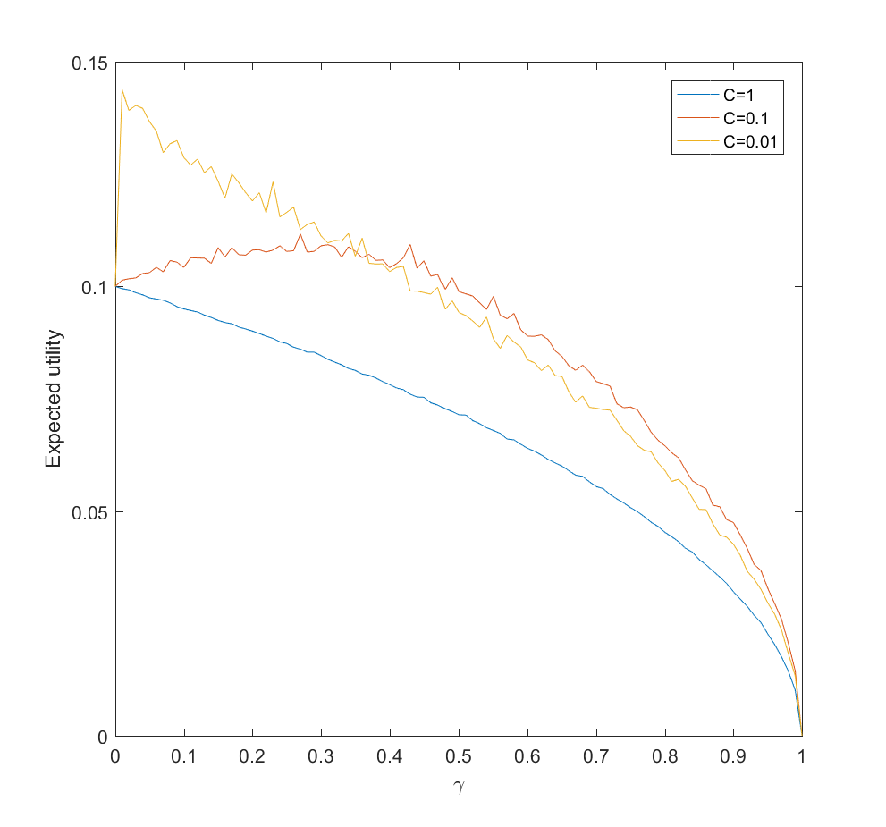
 and the gain is just the utility difference between the uniform case
  , which we know is pretty small. If C is small (i.e. a small amount of effort is enough to figure out the scenario probabilities) there is an optimal nonzero
 , and the center of mass of the polyhedron is just the sum of the simplex centers of mass weighted by their volumes:
  . The volume of a simplex is
 \mathrm{det}(X_j)") where
where ![X_j=[x_{1j};x_{2j};\ldots;x_{Dj}]](https://s0.wp.com/latex.php?latex=X_j%3D%5Bx_%7B1j%7D%3Bx_%7B2j%7D%3B%5Cldots%3Bx_%7BDj%7D%5D&bg=ffffff&fg=000000&s=0 "X_j=[x_{1j};x_{2j};\ldots;x_{Dj}]") , the matrix made by sticking together the coordinate vectors of a simplex. Once we know this we can project the center of mass onto the plane of a face by finding its nullspace (the higher dimensional counterpart to a normal)
, the matrix made by sticking together the coordinate vectors of a simplex. Once we know this we can project the center of mass onto the plane of a face by finding its nullspace (the higher dimensional counterpart to a normal) \vec{n}") . Finally, to check whether the projection is inside the face, we can look at the matrix A where each column is the coordinates of one of the faces minus
. Finally, to check whether the projection is inside the face, we can look at the matrix A where each column is the coordinates of one of the faces minus  and the final row just ones, and solve for Ax=b where b is zero except for a one in the last row (
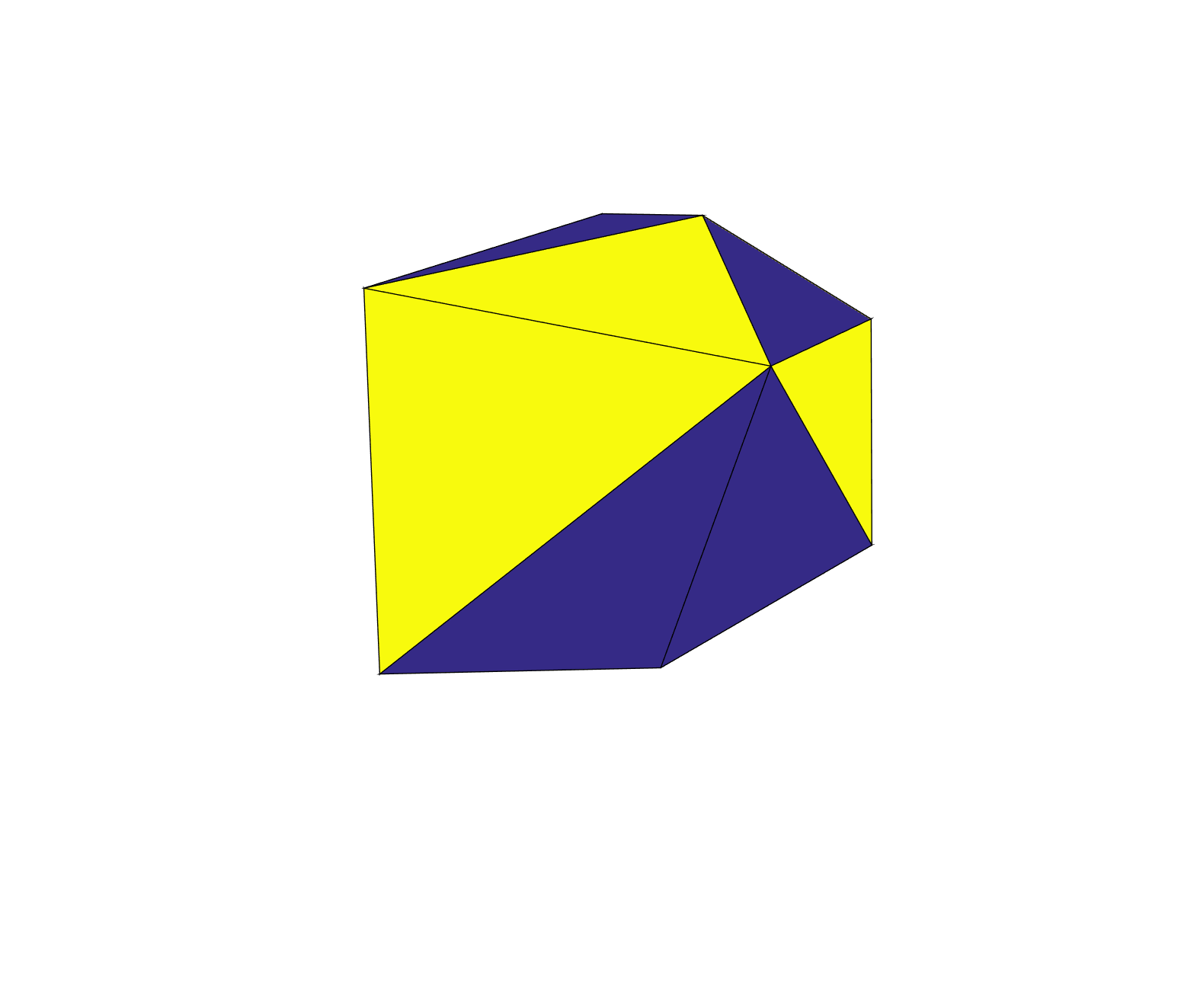

 ), but the number of stable faces also increases exponentially with D (as $latex 2^{0.9273 D}$).
D})=0.8407 D \ln(2) / \ln(D-1) \propto D/\ln(D)") . Even high-dimensional polytopes will stop flipping quickly in general. (A unistable polytope on the other hand can run through at least half of its faces, so there are some very slow ones too).
. Even high-dimensional polytopes will stop flipping quickly in general. (A unistable polytope on the other hand can run through at least half of its faces, so there are some very slow ones too). (if they were optimally distributed it would be
  ). At the same time, if N is relatively small compared to D (the polytope is simplex-like), the average diameter (the longest edge) of each face seems to approach
  . Why? I think this is because
 ") , the mean of a flipped k=2 Weibull distribution that shows up because of
, the mean of a flipped k=2 Weibull distribution that shows up because of  . Faces hence tends to be fairly wide unless N is large compared to D, but there will typically always be a few very narrow ones that are tricky to balance on.
 (or rather, tilt angles – we are doing this in higher dimensions, remember?) generates a hypersphere of radius
 ") around the normal projection point (which is at distance d from the center of mass) where the vertical projection can intersect the face. Only parts of the hypersphere surface that are inside the face represent orientations that are stable. Even an unstable face can (sometimes) be stabilized if you turn it so that the tilted projection is inside, but for sufficiently high angles the hypersphere will be bigger than the face and it cannot be stable.
around the normal projection point (which is at distance d from the center of mass) where the vertical projection can intersect the face. Only parts of the hypersphere surface that are inside the face represent orientations that are stable. Even an unstable face can (sometimes) be stabilized if you turn it so that the tilted projection is inside, but for sufficiently high angles the hypersphere will be bigger than the face and it cannot be stable.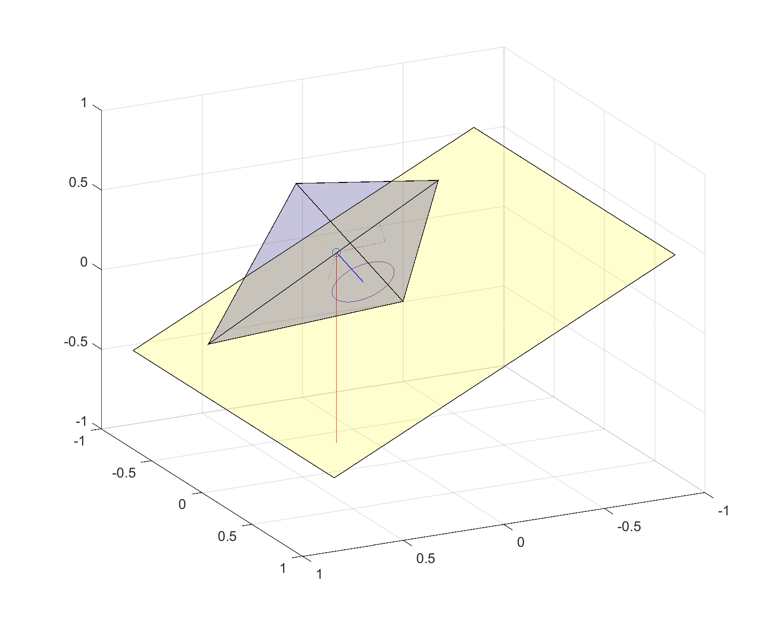
 the first condition might be tougher to meet than the second, but this is just a guess.
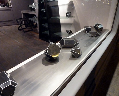
 = Ax(t)/N - px(t-\tau) -x(t)^3")
 is a N-dimensional vector, A is a
  matrix with Gaussian random numbers, and
  constants. The last term should strictly speaking be written as
 ||^2 x(t)") but I am lazy.
but I am lazy. . The final term keeps the dynamics bounded: as
  becomes large this term will dominate and bring back the trajectory to the vicinity of the origin. However, it is a soft spring that has little effect close to the origin.
 . Is it stable? If we calculate the Jacobian matrix there it becomes
  . First, consider the case where
  . The eigenvalues of J will be the ones of a random Gaussian matrix with no symmetry conditions. If it had been symmetric, then
 =(2/\pi)\sqrt{1-\lambda^2}") as
as  . However,
=c_j e^{i\lambda_j t}") into the equation. To simplify, let’s throw away the cubic term since we want to look at behavior close to zero, and let’s use a coordinate system where the matrix is a diagonal matrix
into the equation. To simplify, let’s throw away the cubic term since we want to look at behavior close to zero, and let’s use a coordinate system where the matrix is a diagonal matrix  . Then for
  , that is, the origin is a fixed point that repels or attracts trajectories depending on its eigenvalues (and we know from above that we can be pretty confident some are positive, so it is unstable overall). For
  we get
  . Taylor expansion to the first order and rearranging gives us
 /(1 - i p \tau)") . The numerator means that as
. The numerator means that as  gets large enough it can move the eigenvalue anywhere, causing instability.
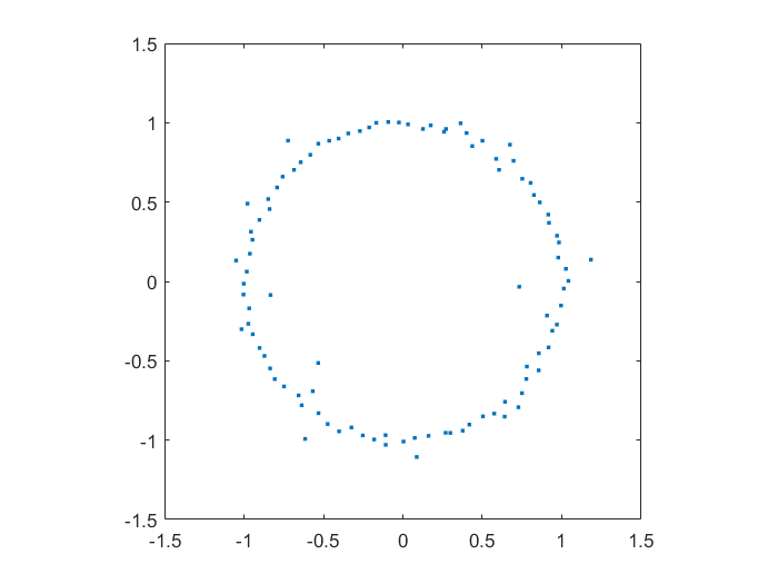
=e^{i\theta} z^n + c_{n-1}z^{n-1}+\ldots+c_1 z + c_0") where
where  were from some suitable random sequence and
 ![[0,2\pi]](https://s0.wp.com/latex.php?latex=%5B0%2C2%5Cpi%5D&bg=ffffff&fg=000000&s=0 "[0,2\pi]") . Since the leading coefficient would start and end up back at 1, I knew all zeros would return to their starting position. But in between, would they jump around discontinuously or follow orderly paths?
. Since the leading coefficient would start and end up back at 1, I knew all zeros would return to their starting position. But in between, would they jump around discontinuously or follow orderly paths? the roots move along different orbits. Some end up permuted with each other.
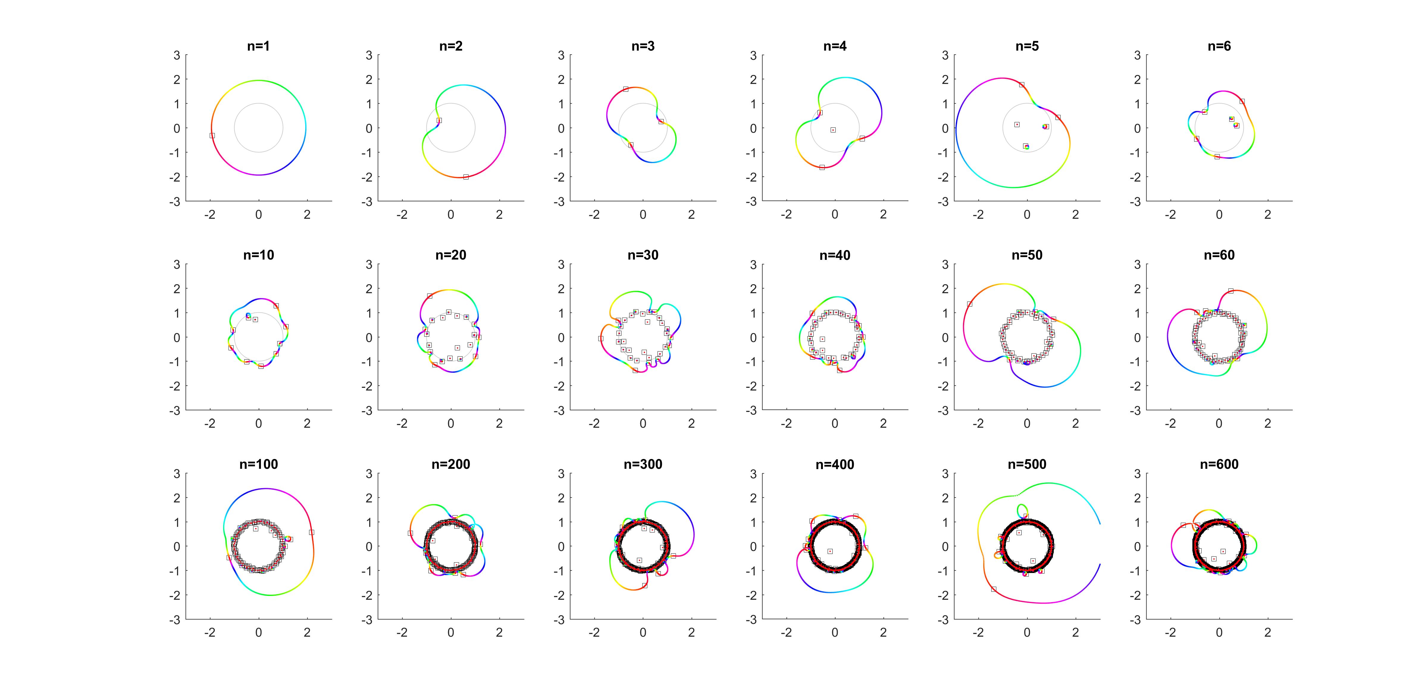
 .
.
 for a r that increases from zero? It turns out that a new zero of the function zooms in from infinity towards the unit circle. A way of seeing this is to look at the polynomial as
  = c_n z^n + P_{n-1}(z)") : the second term is nonzero and large in most places, so if
: the second term is nonzero and large in most places, so if  factor must be large (and opposite) to outweigh it and cause a zero. The exception is of course close to the zeros of
 ") , where the perturbation just moves them a tiny bit: there is a counterpart for each of the
, where the perturbation just moves them a tiny bit: there is a counterpart for each of the  zeros of
 ") . While the new root is approaching from outside, if we play with
. While the new root is approaching from outside, if we play with 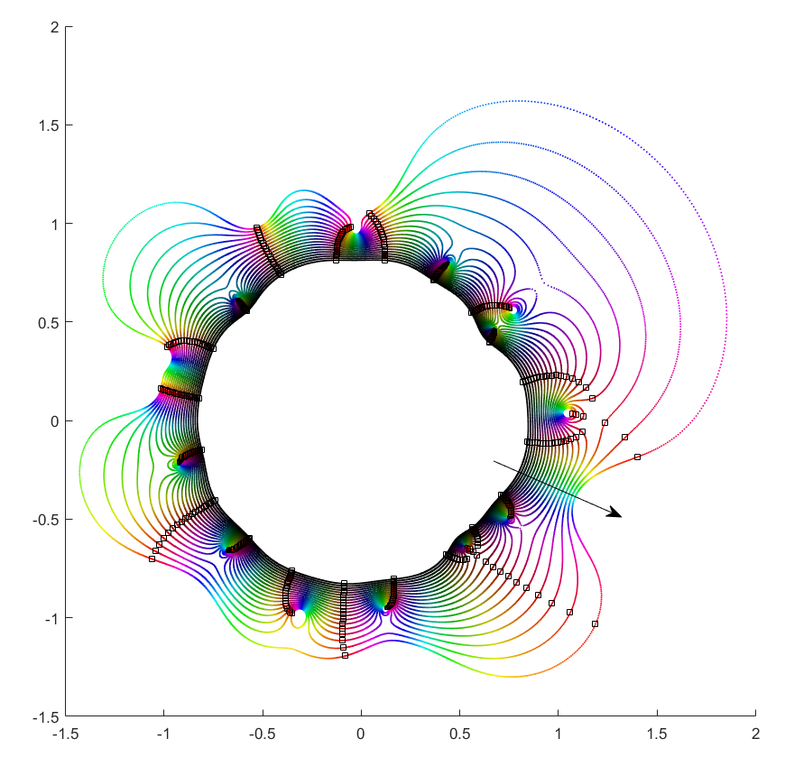
 , then the polynomial is essentially
 ![P_n(z)=c_nz^n+[\mathrm{small stuff}]](https://s0.wp.com/latex.php?latex=P_n%28z%29%3Dc_nz%5En%2B%5B%5Cmathrm%7Bsmall+stuff%7D%5D&bg=ffffff&fg=000000&s=0 "P_n(z)=c_nz^n+[\mathrm{small stuff}]") and the zeros the n-th roots of
and the zeros the n-th roots of ![-[\mathrm{small stuff}]/c_n](https://s0.wp.com/latex.php?latex=-%5B%5Cmathrm%7Bsmall+stuff%7D%5D%2Fc_n&bg=ffffff&fg=000000&s=0 "-[\mathrm{small stuff}]/c_n") . All zeros belong to the same roughly circular orbit, moving together as
. All zeros belong to the same roughly circular orbit, moving together as  decreases the shared orbit develops bulges and dents, and some zeros pinch off from it into their own small circles. When does the pinching off happen? That corresponds to when two zeros coincide during the orbit: one continues on the big orbit, the other one settles down to be local. This is the one case where the analyticity of how they move depending on
  .
. , with
  to
to  separate). That requires a large pinch in the orbit, but since it is overall pretty convex and circle-like this is unlikely.
 to 0 and
  . This is fairly obviously
  = -P_{n-1}(z)/z^n") . This function has a central pole, surrounded by zeros corresponding to the zeros of
. This function has a central pole, surrounded by zeros corresponding to the zeros of |=\mathrm{const}") , and the pinching off to saddle points of this surface. To get a multi-zero orbit several zeros need to be close together enough to cause a broad valley.
, and the pinching off to saddle points of this surface. To get a multi-zero orbit several zeros need to be close together enough to cause a broad valley.
 key ideas needed to produce some important goal (like AI), there is a constant probability per researcher-year to come up with an idea, and the researcher works for
  years, what is the the probability of success? And how does it change if we add more researchers to the team?
=\binom{y}{n}p^n(1-p)^{y-n}") . Unfortunately, then the actual answer to the question will be
. Unfortunately, then the actual answer to the question will be  = \sum_{n=k}^y \binom{y}{n}p^n(1-p)^{y-n}") which is a real mess…
which is a real mess… of good ideas arriving to a researcher, but they can happen at any time. The time between two ideas will be exponentially distributed with parameter
  until a researcher has
 =\lambda^k t^{k-1} e^{-\lambda t} / (k-1)!") .
. (or
(or  ) we will have a good chance of reaching the goal. Unfortunately the variance scales as
  – if the problems are hard, there is a significant risk of being unlucky for a long time. We have to consider the entire distribution.
=1-\sum_{n=0}^{k-1} e^{-\lambda y} (\lambda y)^n / n!") which is again not very nice for algebraic manipulation. Still, we can plot it easily.
which is again not very nice for algebraic manipulation. Still, we can plot it easily. everywhere and get the desired answer.
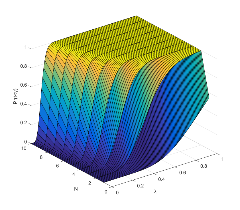
 .
. it rises, and sufficiently above we can be almost certain the project will succeed (the yellow plateau). Conversely, adding extra researchers has decreasing marginal returns when approaching the plateau: they make an already almost certain project even more certain. But they do have increasing marginal returns close to the dark blue “floor”: here the chances of success are small, but extra minds increase them a lot.
 to the one researcher case as we add researchers:
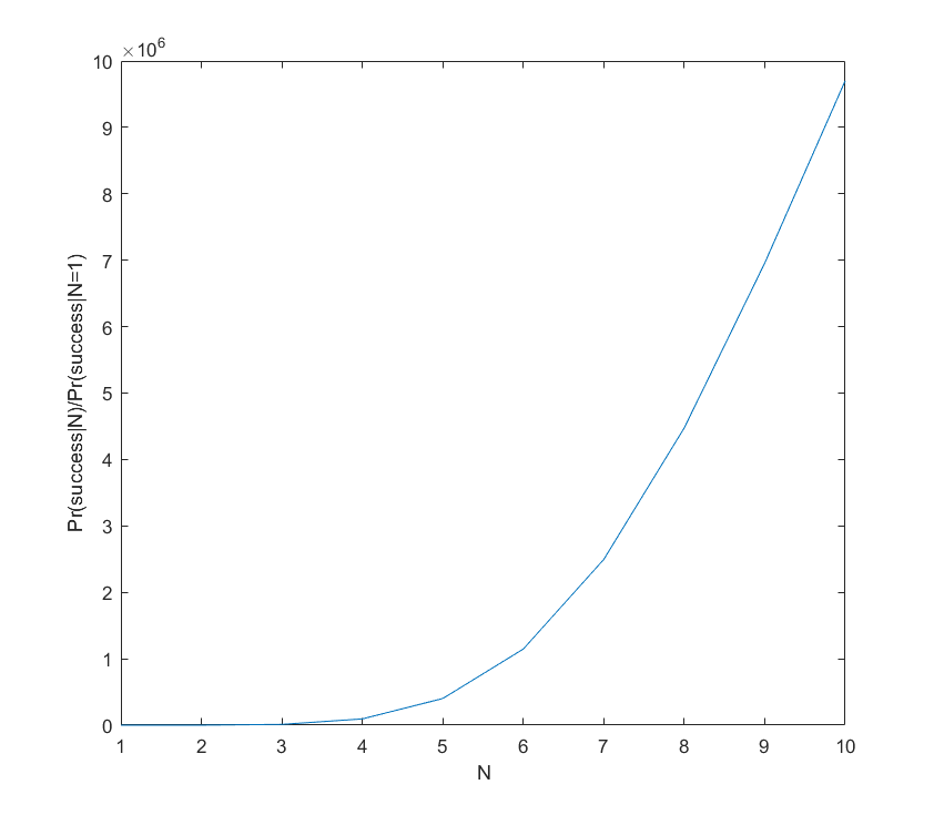
 and how it compares to
  of that idea distributed as an exponential plus the distribution of
 ") . If the first two ideas are independent and exponential with rates
. If the first two ideas are independent and exponential with rates  , then the minimum is distributed as an exponential with rate
  . If they instead require each other, we get a non-exponential distribution (the pdf is
 e^{-(\lambda+\mu)t}") ). Some discoveries or bureaucratic scalings may change the rates. One can construct complex trees of intellectual pathways, unfortunately quickly making the distributions impossible to write out (but still easy to run Monte Carlo on). However, as long as the probabilities and the induced correlations small, I think we can linearise and keep the overall guess that extra minds are exponentially better.
). Some discoveries or bureaucratic scalings may change the rates. One can construct complex trees of intellectual pathways, unfortunately quickly making the distributions impossible to write out (but still easy to run Monte Carlo on). However, as long as the probabilities and the induced correlations small, I think we can linearise and keep the overall guess that extra minds are exponentially better.=z_n^2+c/z_n^3") for some complex constant c. Here are some typical pictures, and two animations: one moving around a circle in the c-plane, one moving slowly down from c=1 to c=0.
for some complex constant c. Here are some typical pictures, and two animations: one moving around a circle in the c-plane, one moving slowly down from c=1 to c=0.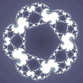
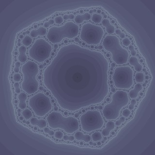
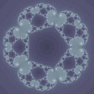
 is clearly mapped to itself. The
  term will tend to make large magnitude iterates approach infinity, so it is an attractive fixed point.
 is a preimage of infinity: iterates falling on zero will be mapped onto infinity. Nearby points will also end up attracted to infinity, so we have a basin of attraction to infinity around the origin. Preimages of the origin will be mapped to infinity in two steps:
  has the solutions
 ^{1/5}") – this is where the pentagonal symmetry comes from, since these five points are symmetric. Their preimages and so on will also be mapped to infinity, so we have a hierarchy of basins of attraction sending points away forming some gasket-like structure. The Julia set consists of the points that never gets mapped away, the boundary of this hierarchy of basins.
– this is where the pentagonal symmetry comes from, since these five points are symmetric. Their preimages and so on will also be mapped to infinity, so we have a hierarchy of basins of attraction sending points away forming some gasket-like structure. The Julia set consists of the points that never gets mapped away, the boundary of this hierarchy of basins. , which can be rearranged into
  . They don’t have any neat expression and actually do not affect the big picture dynamics as much. The main reason seems to be that they are unstable. However, their location and the derivative close to them affect the shapes in the Julia set as we will see. Their preimages will be surrounded by the same structures (scaled and rotated) as they have.
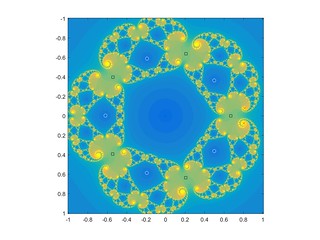
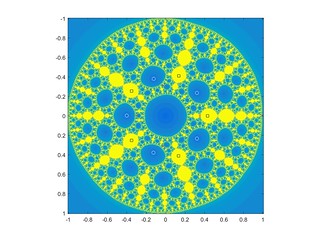
^{1/5}") and mapping out its fate in the c-plane. Why that particular point? Because it is one of the critical point where
and mapping out its fate in the c-plane. Why that particular point? Because it is one of the critical point where =0") , and a theorem by Julia and Fatou tells us that its fate indicates whether the Julia set is filled or dust-like: bounded orbits of the critical points of a map imply a connected Julia set. When c is in the Mandelbrot set the Julia image has “thick” regions with finite area that do not escape to infinity. When c is outside, then most points end up at infinity, and what remains is either dust or a thin gasket with no area.
, and a theorem by Julia and Fatou tells us that its fate indicates whether the Julia set is filled or dust-like: bounded orbits of the critical points of a map imply a connected Julia set. When c is in the Mandelbrot set the Julia image has “thick” regions with finite area that do not escape to infinity. When c is outside, then most points end up at infinity, and what remains is either dust or a thin gasket with no area.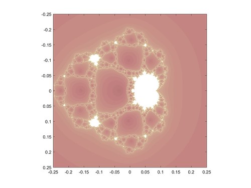
=z^2+c") Mandelbrot, with a cuspy main body surrounded by a net reminiscent of the gaskets in the Julia set. It also has satellite vanilla Mandelbrots,
Mandelbrot, with a cuspy main body surrounded by a net reminiscent of the gaskets in the Julia set. It also has satellite vanilla Mandelbrots, 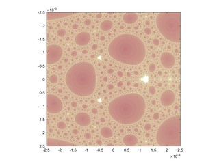
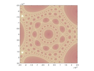
 . Looking at the dynamics, above this point the iterates of the critical point jump around in the interval [0,1], forming a typical Feigenbaum cascade of period doubling as you go out along the spar (just like on the spar of the vanilla Mandelbrot set). But at this location points now are mapped outside the interval, running off to infinity: one of the critical points breaches a basin boundary, causing iterates to run off and the earlier separate basins to merge. Below this point the dynamics is almost completely dominated by the squaring, turning the Julia set into a product of a Cantor set and a circle (a bit wobbly for higher c; it is all very similar to
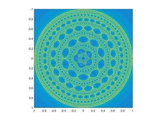
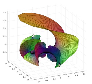
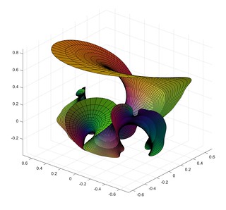
=\sum_{p \mathrm{is prime}} z^p") , the Taylor series that only includes all prime powers, combined with
, the Taylor series that only includes all prime powers, combined with =1") .
.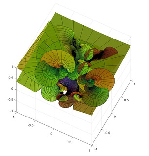
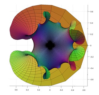
 ), you formally define a function
 =\sum_{n=0}^\infty a_n z^n") , you derive some constraints on the function, and from this you get a formula for the
, you derive some constraints on the function, and from this you get a formula for the ") seriously as a (complex) function and use the powerful machinery of complex analysis to calculate asymptotic behavior for the
seriously as a (complex) function and use the powerful machinery of complex analysis to calculate asymptotic behavior for the 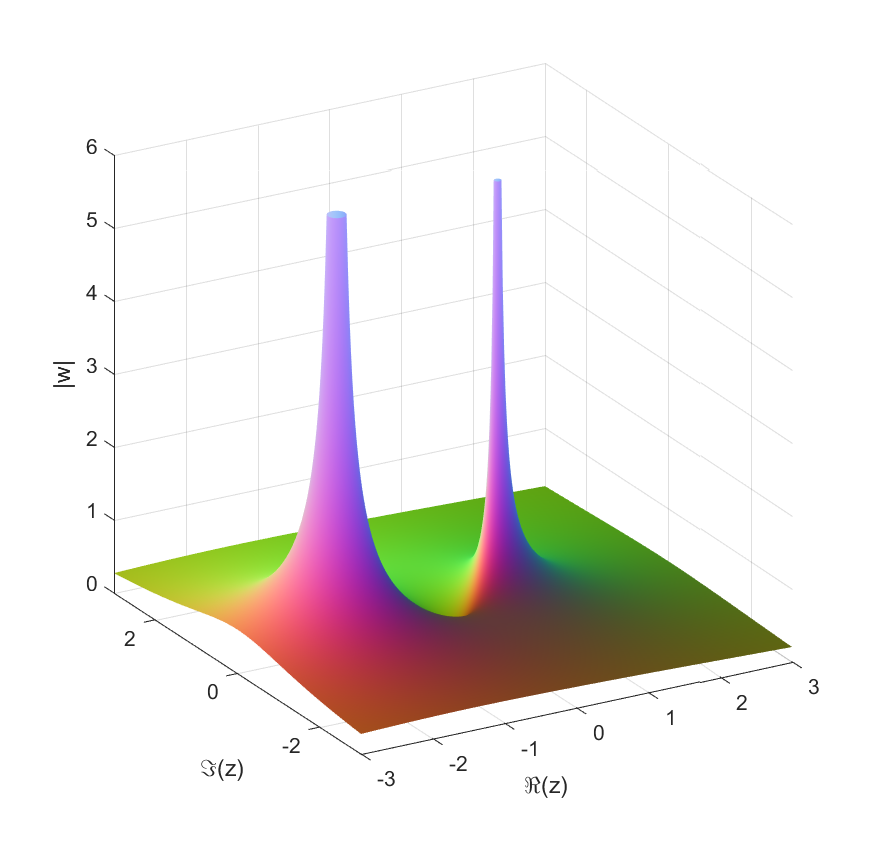
 , while single tuck tie knots grow as
  .
.=\sum_{n=0}^\infty X_n z^n") where
where  are independent random numbers, what kind of functions do we get? Trying it with complex Gaussian
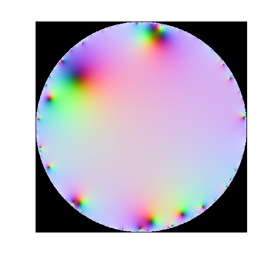
 we have an exponentially decaying sequence of
 ") and not too divergent variance we should expect convergence, while outside the unit circle any nonzero
and not too divergent variance we should expect convergence, while outside the unit circle any nonzero  \leq E(X)/t") to argue that a series
to argue that a series ") would converge if
would converge if /n") converges. However, this is not correct enough for proper mathematics. One entirely possible Gaussian outcome is
converges. However, this is not correct enough for proper mathematics. One entirely possible Gaussian outcome is  or worse. We need to speak of probabilistic convergence.
 of an uncontinuable function). In fact,