My view is largely that moral action is strongly driven and motivated by emotions rather than reason, but outside the world of the blindingly obvious or everyday human activity our intuitions and feelings are not great guides. We do not function well morally when the numbers get too big or the cognitive biases become maladaptive. Morality may be about the heart, but ethics is in the brain.
It is a delightful little spin/parody of Searle’s original, bringing up questions of what constitutes sex, consent and relationships, and quite nicely illuminates some of the issues with technologically mediated human interaction.
This kind of prank is of course by why naive keyword-based watch lists are total failures. One prank and it gets overloaded. I would be shocked if any serious intelligence agency actually used them for real. Given that people’s Facebook likes give pretty good predictions of who they are (indeed, better than many friends know them) there are better methods if you happen to be a big intelligence agency.
Still, while text and other online behavior signal a lot about a person, it might not be a great tool for making proper watchlists since there is a lot of noise. For example, this paper extracts personality dimensions from online texts and looks at civilian mass murderers. They state:
Using this ranking procedure, it was found that all of the murderers’ texts were located within the highest ranked 33 places. It means that using only two simple measures for screening these texts, we can reduce the size of the population under inquiry to 0.013% of its original size, in order to manually identify all of the murderers’ texts.
At first, this sounds great. But for the US, that means the watchlist for being a mass murderer would currently have 41,000 entries. Given that over the past 150 years there has been about 150 mass murders in the US, this suggests that the precision is not going to be that great – most of those people are just normal people. The base rate problem crops up again and again when trying to find rare, scary people.
The deep problem is that there is not enough positive data points (the above paper used seven people) to make a reliable algorithm. The same issue cropped up with NSA’s SKYNET program – they also had seven positive examples and hundreds of thousands of negatives, and hence had massive overfitting (suggesting the Islamabad Al Jazeera bureau chief was a prime Al Qaeda suspect).
Rational watchlists
The rare positive data point problem strikes any method, no matter what it is based on. Yes, looking at the social network around people might give useful information, but if you only have a few examples of bad people the system will now pick up on networks like the ones they had. This is also true for human learning: if you look too much for people like the ones that in the past committed attacks, you will focus too much on people like them and not enemies that look different. I was told by an anti-terrorism expert about a particular sign for veterans of Afghan guerrilla warfare: great if and only if such veterans are the enemy, but rather useless if the enemy can recruit others. Even if such veterans are a sizable fraction of the enemy the base rate problem may make you spend your resources on innocent “noise” veterans if the enemy is a small group. Add confirmation bias, and trouble will follow.
Note that actually looking for a small set of people on the watchlist gets around the positive data point problem: the system can look for them and just them, and this can be made precise. The problem is not watching, but predicting who else should be watched.
The point of a watchlist is that it represents a subset of something (whether people or stocks) that merits closer scrutiny. It should essentially be an allocation of attention towards items that need higher level analysis or decision-making. The U.S. Government’s Consolidated Terrorist Watch List requires nomination from various agencies, who presumably decide based on reasonable criteria (modulo confirmation bias and mistakes). The key problem is that attention is a limited resource, so adding extra items has a cost: less attention can be spent on the rest.
This is why automatic watchlist generation is likely to be a bad idea, despite much research. Mining intelligence to help an analyst figure out if somebody might fit a profile or merit further scrutiny is likely more doable. As long as analyst time is expensive it can easily be overwhelmed if something fills the input folder: HUMINT is less likely to do it than SIGINT, even if the analyst is just doing the preliminary nomination for a watchlist.
The optimal Bayesian watchlist
One can analyse this in a Bayesian framework: assume each item has a value distributed as . The goal of the watchlist is to spend expensive investigatory resources to figure out the true values; say the cost is 1 per item. Then a watchlist of randomly selected items will have a mean value . Suppose a cursory investigation costing much less gives some indication about , so that it is now known with some error: . One approach is to select all items above a threshold , making .
If we imagine that everything is Gaussian , then . While one can ram through this using Owen’s useful work, here is a Monte Carlo simulation of what happens when we use (the correlation between x and y is 0.707, so this is not too much noise):
Utility of selecting items for watchlist as a function of threshold. Red curve without noise, blue with N(0,1) noise added.
Note that in this case the addition of noise forces a far higher threshold than without noise (1.22 instead of 0.31). This is just 19% of all items, while in the noise-less case 37% of items would be worth investigating. As noise becomes worse the selection for a watchlist should become stricter: a really cursory inspection should not lead to insertion unless it looks really relevant.
Here we used a mild Gaussian distribution. In term of danger, I think people or things are more likely to be lognormal distributed since it is a product of many relatively independent factors. Using lognormal x and y leads to a situation where there is a maximum utility for some threshold. This is likely a problematic model, but clearly the shape of the distributions matter a lot for where the threshold should be.
Note that having huge resources can be a bane: if you build your watchlist from the top priority down as long as you have budget or manpower, the lower priority (but still above threshold!) entries will be more likely to be a waste of time and effort. The average utility will decline.
Predictive validity matters more?
In any case, a cursory and cheap decision process is going to give so many so-so evaluations that one shouldn’t build the watchlist on it. Instead one should aim for a series of filters of increasing sophistication (and cost) to wash out the relevant items from the dross.
We find that when searching for rare positives (e.g., candidates that will successfully complete clinical development), changes in the predictive validity of screening and disease models that many people working in drug discovery would regard as small and/or unknowable (i.e., an 0.1 absolute change in correlation coefficient between model output and clinical outcomes in man) can offset large (e.g., 10 fold, even 100 fold) changes in models’ brute-force efficiency.
Just like for drugs (an example where the watchlist is a set of candidate compounds), it might be more important for terrorist watchlists to aim for signs with predictive power of being a bad guy, rather than being correlated with being a bad guy. Otherwise anti-terrorism will suffer the same problem of declining productivity, despite ever more sophisticated algorithms.
I recently nerded out about high-energy proton interaction with matter, enjoying reading up on the Bethe equation at the Particle Data Group review and elsewhere. That got me to look around at the PDL website, which is full of awesome stuff – everything from math and physics reviews to data for the most obscure “particles” ever, plus tests of how conserved the conservation laws are.
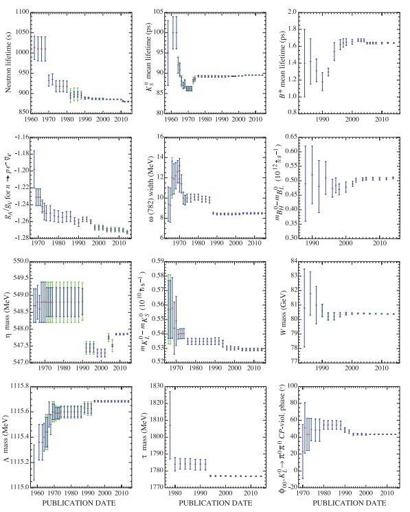
Historical graph of physical constant estimates from K.A. Olive et al. (Particle Data Group), Chin. Phys. C, 38, 090001 (2014) and 2015 update.
The first thing that strikes the viewer is that they have moved a fair bit, including often being far outside the original error bars. 6 of them have escaped them. That doesn’t look very good for science!
Fortunately, it turns out that these error bars are not 95% confidence intervals (the most common form in many branches of science) but 68.3% confidence intervals (one standard deviation, if things are normal). That means having half of them out of range is entirely reasonable! On the other hand, most researchers don’t understand error bars (original paper), and we should be able to do much better.
Sometimes large changes occur. These usually reflect the introduction of significant new data or the discarding of older data. Older data are discarded in favor of newer data when it is felt that the newer data have smaller systematic errors, or have more checks on systematic errors, or have made corrections unknown at the time of the older experiments, or simply have much smaller errors. Sometimes, the scale factor becomes large near the time at which a large jump takes place, reflecting the uncertainty introduced by the new and inconsistent data. By and large, however, a full scan of our history plots shows a dull progression toward greater precision at central values quite consistent with the first data points shown.
Overall, kudos to PDG for showing the history and making it clearer what is going on! But I do not agree it is a dull progression.
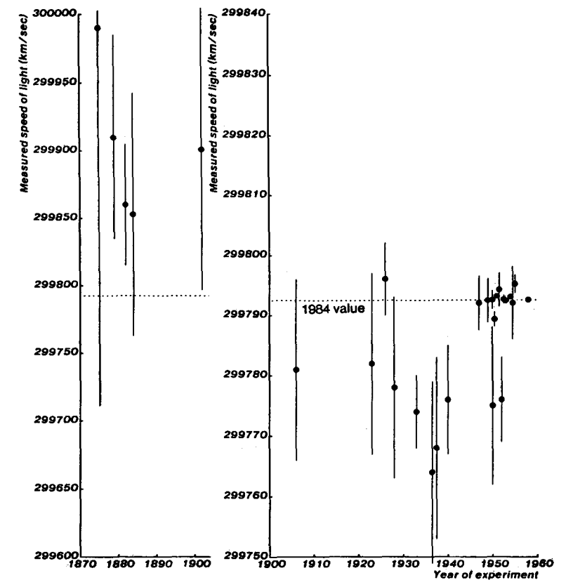
Plot of light-speed measurements 1875-1958. Error bars are standard error. From Max Henrion and Baruch Fischhoff. Assessing uncertainty in physical constants. American Journal of Physics 54, 791 (1986); doi: 10.1119/1.14447.
Note that the shifts were far larger than the estimated error bars. The dip in the 1930s and 40s even made some physicists propose that c could be changing over time. Overall Henrion and Fischhoff find that physicists have been rather overconfident in their tight error bounds on their measurements. The approach towards current estimates is anything but dull, and hides many amusing historical anecdotes.
Stories like this might have been helpful; it is notable that the PDG histories on the right, for newer constants, seem to stay closer to the present value than the longer ones to the left. Maybe this is just because they have not had the time to veer off yet, but one can be hopeful.
Still, even if people are improving this might not mean the conclusions stay stable or approach truth monotonically. A related issue is “negative learning”, where more data and improved models make the consensus view of a topic move in the wrong direction: Oppenheimer, M., O’Neill, B. C., & Webster, M. (2008). Negative learning. Climatic Change, 89(1-2), 155-172. Here the problem is not just that people are overconfident in how certain they can be about their conclusions, but also that there is a bit of group-think, plus that the models change in structure and are affected in different ways by the same data. They point out how estimates of ozone depletion oscillated, or the consensus on the stability of climate has shifted from oscillatory (before 1968) towards instability (68-82), towards stability (82-96), and now towards instability again (96-06). These problems are not due to mere irrationality, but the fact that as we learn more and build better models these incomplete but better models may still deviate strongly from the ground truth because they miss some key component.
Noli fumare
This is related to what Nick Bostrom calls the “data fumes” problem. Early data will be fragmentary and explanations uncertain – but the data points and their patterns are very salient, just as the early models, since there is nothing else. So we begin to anchor on them. Then new data arrives and the models improve… and the old patterns are revealed as statistical noise, or bugs in the simulation or plotting routine. But since we anchored on them, we are unlikely to update as strongly towards the new most likely estimates. Worse, accommodating a new model takes mental work; our status quo bias will be pushing against the update. Even if we do accommodate the new state, things will likely change more – we may well end up either with a view anchored on early noise, or assume that the final state is far more uncertain than it actually is (since we weigh the early jumps strongly because of their saliency).
This is of course why most people prefer to believe a charismatic diet cultleader expert rather than trying to dig through 70 years of messy, conflicting dietary epidemiology.
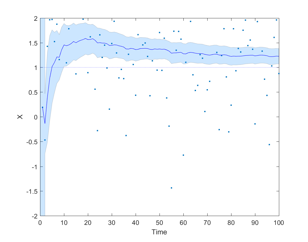
Here is a simple example where an agent is trying to do a maximum likelihood estimation of a Gaussian distribution with mean 1 and variance 1, but is hamstrung by giving double weight to the first 9 data points:
Simple data fume model, showing the slow and biased convergence when the first 9 data points are over-weighted. The blue area is a 95% confidence interval for the mean of the generating Gaussian distribution.
It is not hard to complicate the model with anchoring/recency/status quo bias (estimates get biased towards previous estimates), or that early data points are more polluted by differently distributed noise. Asymmetric error checking (you will look for bugs if results deviate from expectation and hence often find such bugs, but not look for bugs making your results closer to expectation) is another obvious factor for how data fumes can get integrated in models.
The problem with data fumes is that it is not easy to tell when you have stabilized enough to start trusting the data. It is even messier when the inputs are results generated by your own models or code. I like to approach it by using multiple models to guesstimate model error: for example, one mathematical model on paper and one Monte Carlo simulation – if they don’t agree, then I should disregard either answer and keep on improving.
Even when everything seems to be fine there may be a big crucial consideration one has missed. The Turing-Good estimator gives another way of estimating the risk of that: if you have acquired data points and seen big surprises (remember that the first data point counts as one!), then the probability of a new surprise for your next data point is . So if you expect data points in total, when you can start to trust the estimates… assuming surprises are uncorrelated etc. Which you will not be certain about. The progression towards greater precision may be anything but dull.
In Scott Alexander’s kabbalistic sf story Unsong, the archangel Uriel works on a problem while other things are going on in heaven:
All the angels listened in rapt attention except Uriel, who was sort of half-paying attention while trying to balance several twelve-dimensional shapes on top of each other.
…
There was utter silence throughout the halls of Heaven, except a brief curse as Uriel’s hyperdimensional tower collapsed on itself and he picked up the pieces to try to rebuild it.
…
A great clamor arose from all the heavenly hosts, save Uriel, who took advantage of the brief lapse to conjure a parchment and pen and start working on a proof about the optimal configuration of twelve-dimensional shapes.
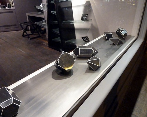
This got me thinking about the stability of stacking polytopes. That seemed complicated (I am no archangel) so I started toying with the stability of polytopes on a flat surface.
(Terminology note: I will consistently use “face” to denote the D-1 dimensional elements that bound the polytope, although “facet” is in some use.)
A face of a 3D polyhedron is stable if the polyhedron can rest on it without tipping over. This means that the projection of the center of mass onto the plane containing the face is inside the polygon. The platonic polyhedra are stable on all faces, but it is not hard to make a few faces unstable by moving a vertex far away from the center. A polyhedron has at least one stable face (if it did not, it would be a perpetual motion device: every tip will move the center of mass downwards, but there is a bound on how low it can go. A uni-stable or monostatic polyhedron has just one stable face. It is an unsolved problem what the simplest uni-stable 3D polyhedron is, with the current record 14 faces. Also, it seems unclear whether there are monostatic simplices in dimension 9 (they exist in 10 or more dimensions, but not in 8 or fewer).
So, how many faces of a polytope will typically be unstable?
I wrote a Matlab script to generate random convex polytopes by selecting N points randomly on the surface of a D-dimensional sphere and calculating their convex hull. Using a Delaunay decomposition I can split them into simplices, which allow me to calculate the center of mass. The center of mass of a simplex is just the average of the corners , and the center of mass of the polyhedron is just the sum of the simplex centers of mass weighted by their volumes: . The volume of a simplex is where , the matrix made by sticking together the coordinate vectors of a simplex. Once we know this we can project the center of mass onto the plane of a face by finding its nullspace (the higher dimensional counterpart to a normal) . Finally, to check whether the projection is inside the face, we can look at the matrix A where each column is the coordinates of one of the faces minus and the final row just ones, and solve for Ax=b where b is zero except for a one in the last row (I found this neat algorithm due to elisbben on stack overflow). If the answer vector is all positive, then the point is inside the face. Repeat for all the faces.
Whew. This math is of course really simple to do in Matlab.
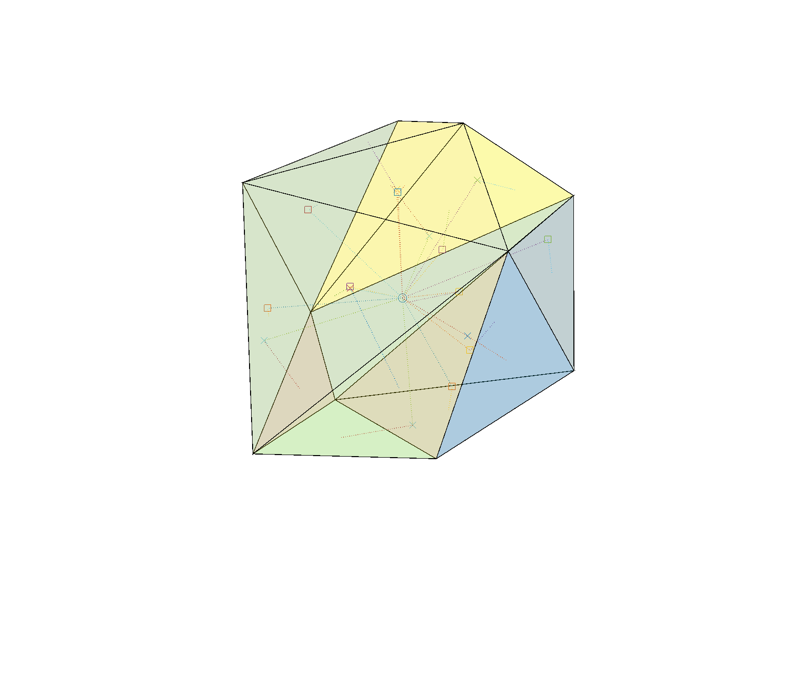
Stable (yellow) and unstable (blue) faces of random polyhedron.Stability of random polyhedron. The center of mass is marked by a circle. It is projected along the dotted lines into the plane of each face, marked with a square (if inside the face and hence a stable face) or a cross (if outside the face, which is hence unstable). A dotted line connects the projection points to the center of their face.
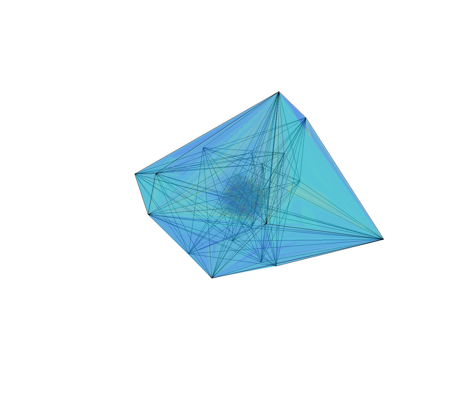
The 12 dimensional case is a bit messier:
Projection of a 12D polytope with 20 vertices. Each of the 2777 faces is a 11 dimensional simplex.
So, what is the average fraction of stable faces on a 3D polyhedron?
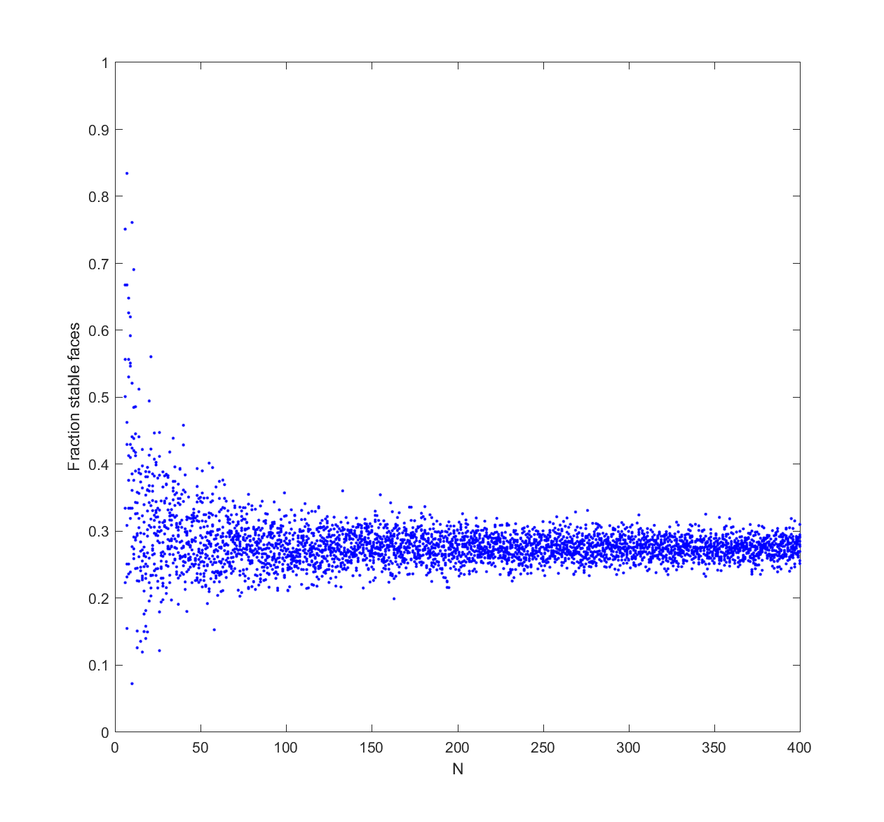
Fraction stable faces on 3D convex hulls of N points on a sphere.
It tends to converge to 50%. Doing this in higher dimensions shows the same kind of convergence, although to lower fractions.
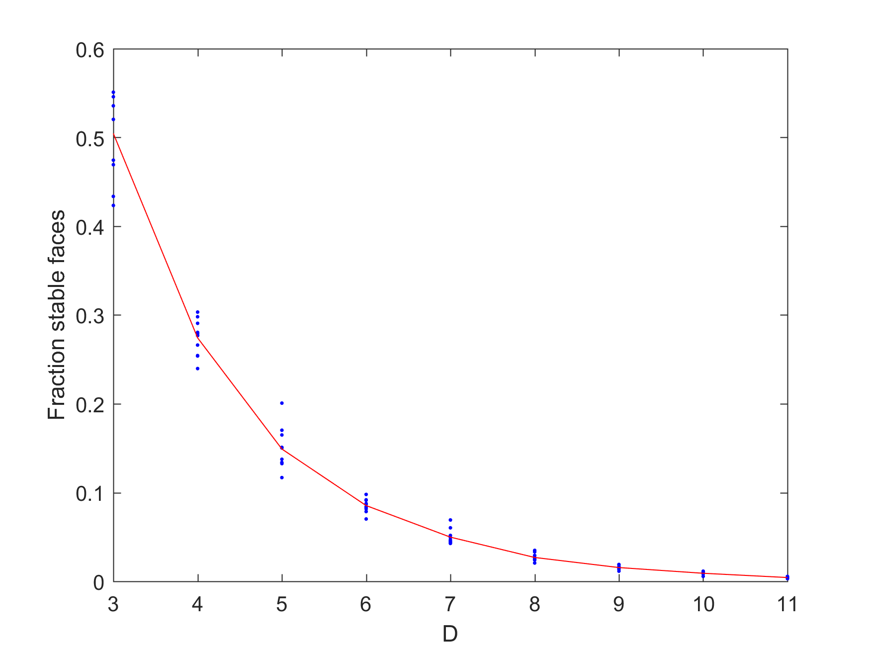
Fraction stable faces on 4D convex hulls of N points on a sphere.Fraction stable faces of N=100 convex hulls in different dimensions. Red line exponential fit.
It looks like the fraction of stable faces declines exponentially with dimensionality.
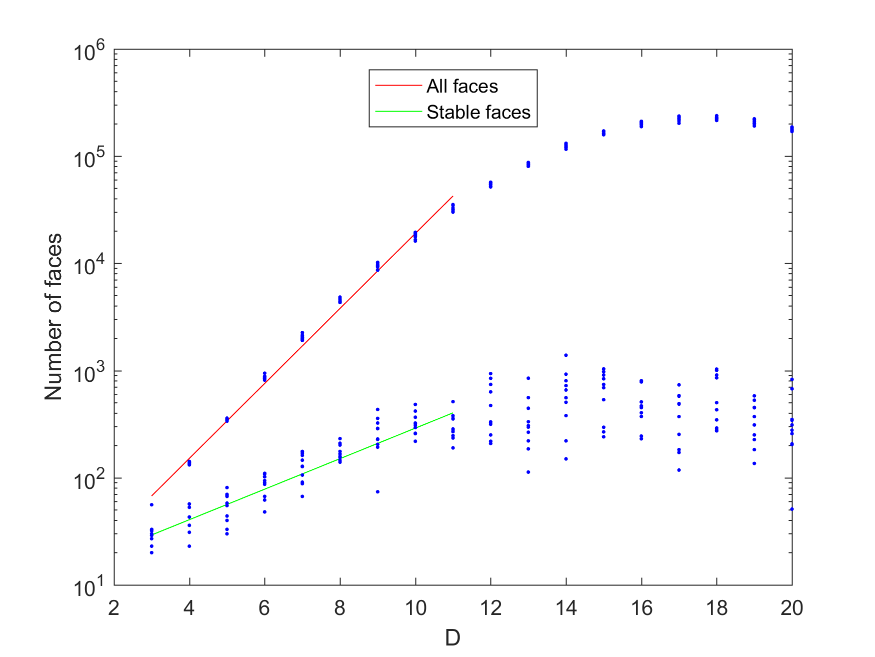
Does this mean that for a sufficiently high dimension it is likely that a random polytope is unistable? The answer is no: the number of faces increases pretty exponentially (as ), but the number of stable faces also increases exponentially with D (as $latex 2^{0.9273 D}$).
Combined plot of number of faces (points with red line) and stable faces (points with green line) as a function of dimension for N=100.
This was based on runs with N=100. Obviously things go much faster if you select a lower N, such as 30. However, as you approach N=D the polytopes become more and more simplex-like, and simplices tend to both have fewer faces and be less stable in high dimensions, so the exponential growth stops. This actually happens far below D; for N=30 the effect is felt already in 11 dimensions. The face growth rates were also lower, with coefficients 1.1621 and 0.4730.
Number of faces and stable faces for N=30 random convex hulls in different dimensions.
(There are some asymptotic formulas known for the growth of the number of faces for random convex hulls; they grow linearly with N but at an accelerating rate with D.)
Stuart Armstrong gave me a very heuristic argument for why there would be so many unstable faces. Consider building up the polytope vertex by vertex, essentially just adding together the simplices from the Delaunay decomposition. If you start from a stable state, eventually you will likely end up with an unstable face. Adding the next vertex will add a simplex to the polyhedron, and the center of mass will move in the direction of the new simplex. To have the face become stable again the shift in center of mass needs to be large enough along the directions parallel to the face to bring the projection back inside the face. But in high dimensional spaces there are many directions you can move in: the probability of a random vector being nearly parallel to another vector is very low. Hence, the next step and the following are likely to preserve the instability. So high dimensional polytopes are likely to have many unstable faces even if they are nicely inscribed in spheres.
The number of steps the polytope rolls over until finding a stable face is also limited: the “drainage basin” of a stable face is a tree, with a branching degree set by D-1 (if faces are D-simplexes). So the number of steps will scale as . Even high-dimensional polytopes will stop flipping quickly in general. (A unistable polytope on the other hand can run through at least half of its faces, so there are some very slow ones too).
The expected minimum distance between two points on this kind of random polytope scales as (if they were optimally distributed it would be ). At the same time, if N is relatively small compared to D (the polytope is simplex-like), the average diameter (the longest edge) of each face seems to approach . Why? I think this is because , the mean of a flipped k=2 Weibull distribution that shows up because of extreme value theory. Meanwhile the average and median cord length between random points on hyperspheres tends towards . Faces hence tends to be fairly wide unless N is large compared to D, but there will typically always be a few very narrow ones that are tricky to balance on.
Stacking no-slip polytopes
What about stacking polytopes?
If you put a polytope on top of another one (assuming no slipping) at first it seems you need to use a stable face of the top polytope, but this is not enough nor necessary.
Since the underlying face is likely tilted from the horizontal, the vertical projection of the center of mass has to be within the top face. The upper polytope can be rotated, moving the projection point. The tilt angle (or rather, tilt angles – we are doing this in higher dimensions, remember?) generates a hypersphere of radius around the normal projection point (which is at distance d from the center of mass) where the vertical projection can intersect the face. Only parts of the hypersphere surface that are inside the face represent orientations that are stable. Even an unstable face can (sometimes) be stabilized if you turn it so that the tilted projection is inside, but for sufficiently high angles the hypersphere will be bigger than the face and it cannot be stable.
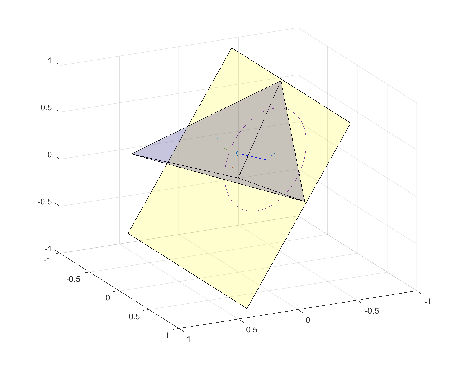
Stability of polyhedron on tilted surface. The line of gravity from the center of mass intersects the inside the bottom face, so the polyhedron is resting stably. Turning the polyhedron will move the line to some point on the circle, but since all points on the circle are inside the face all orientations are stable.Stability of polyhedron on tilted surface. The line of gravity from the center of mass intersects the outside the bottom face, so the polyhedron is unstable and will flip over. Turning the polyhedron will move the line to some other point on the circle: since some points on the circle are inside the face there are some orientations that are stable.
Having the top polytope stay in place is the first requirement. The second is that the bottom polytope should not become unstable. The new center of mass is moved to a point somewhere along the connecting line between the individual centers of mass of the polytopes, with exact position dependent on their volume ratio (note that turning the top polytope can move the center of mass too). This moves the projection point along the plane of the bottom face, and if it gets outside that face the assembly will tip over.
One can imagine this as adding random (D-1)-dimensional vectors of length 1/N until they reach the edge of the face. I am a bit uncertain about the properties of such random walks (all works on decreasing step size walks I have seen have been in 1D). The harmonic random walk in 1D apparently converges with probability 1, so I think the (D-1)-dimensional one also does it since the distance from the origin to the walker will be smaller than if the walker just kept to a 1D line. Since the expected distance traversed in 1D is $latex E[|X|] \approx 1.0761$ this is actually not a very extreme shift. Given the surprisingly large diameters of the faces if the first condition might be tougher to meet than the second, but this is just a guess.
The no slipping constraint is important. If the polytopes are frictionless, then any transverse force will move them. Hence only polytopes that have some parallel top and bottom stable faces can be stacked, and the problem becomes simpler. There are still surprises there, though: even stacks of rectangular blocks can do surprising things. The block stacking problem also demonstrates that one can have 1/N overhangs (counting downwards), enabling arbitrarily large total overhangs without tipping over. With polytopes with shapes that act as counterweights the overhangs can be even larger.
Uriel’s stacking problems
This leads to what we might call “Uriel’s stacking problem”: given a collection of no-slip convex D-dimensional polytopes, what is the tallest tower that can be constructed from them?
I suspect that this problem is NP-hard. It sounds very much like a knapsack problem, but there is a dependency on previous steps when you add a new polytope that seem to make it harder. It seems that it would not be too difficult to fool a greedy algorithm just trying to put the next polytope on the most topmost face into adding one that makes subsequent steps too unstable, forcing backtracking.
Another related problem: if the polytopes are random convex hulls of N points, what is the distribution of maximum tower heights? What if we just try random stacking?
And finally, what is the maximum overhang that can be done by stacking polytopes from a given set?
Were robots thinking, moral beings liability would be easy: they would presumably be legal subjects and handled like humans and corporations. But now they have an uneasy position as legal objects yet endowed with the ability to perform complex actions on behalf of others, or with emergent behaviors nobody can predict. The challenge may be to design not just the robots or laws, but robots and laws that fit each other (and real social practices): social robotics.
But it is early days. It is actually hard to tell where robotics will truly shine or matter legally, and premature laws can stifle innovation. We also do not really know what principles we ought to use to underpin the social robotics – more research is needed. And if you thought AI safety was hard, now consider getting machines to fit into the even less well defined human social landscape.
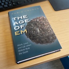
Robin Hanson’s The Age of Em is bound to be a classic.
It might seem odd, given that it is both awkward to define what kind of book it is – economics textbook, future studies, speculative sociology, science fiction without any characters? – and that most readers will disagree with large parts of it. Indeed, one of the main reasons it will become classic is that there is so much to disagree with and those disagreements are bound to stimulate a crop of blogs, essays, papers and maybe other books.
This is a very rich synthesis of many ideas with a high density of fascinating arguments and claims per page just begging for deeper analysis and response. It is in many ways like an author’s first science fiction novel (Zindell’s Neverness, Rajaniemi’s The Quantum Thief, and Egan’s Quarantine come to mind) – lots of concepts and throwaway realizations has been built up in the background of the author’s mind and are now out to play. Later novels are often better written, but first novels have the freshest ideas.
The second reason it will become classic is that even if mainstream economics or futurism pass it by, it is going to profoundly change how science fiction treats the concept of mind uploading. Sure, the concept has been around for ages, but this is the first through treatment of what it means to a society. Any science fiction treatment henceforth will partially define itself by how it relates to the Age of Em scenario.
Plausibility
The Age of Em is all about the implications of a particular kind of software intelligence, one based on scanning human brains to produce intelligent software entities. I suspect much of the debate about the book will be more about the feasibility of brain emulations. To many people the whole concept sparks incredulity and outright rejection. The arguments against brain emulation range from pure arguments of incredulity (“don’t these people know how complex the brain is?”) over various more or less well-considered philosophical positions (“don’t these people read Heidegger?” to questioning the inherent functionalist reductionism of the concept) to arguments about technological feasibility. Given that the notion is one many people will find hard to swallow I think Robin spent too little effort bolstering the plausibility, making the book look a bit too much like what Nordmann called if-then ethics: assume some outrageous assumption, then work out the conclusion (which Nordmann finds a waste of intellectual resources). I think one can make fairly strong arguments for the plausibility, but Robin is more interested in working out the consequences. I have a feeling there is a need now for a good defense of the plausibility (this and this might be a weak start, but much more needs to be done).
Scenarios
In this book, I will set defining assumptions, collect many plausible arguments about the correlations we should expect from these assumptions, and then try to combine these many correlation clues into a self-consistent scenario describing relevant variables.
What I find more interesting is Robin’s approach to future studies. He is describing a self-consistent scenario. The aim is not to describe the most likely future of all, nor to push some particular trend the furthest it can go. Rather, he is trying to describe what, given some assumptions, is likely to occur based on our best knowledge and fits with the other parts of the scenario into an organic whole.
The baseline scenario I generate in this book is detailed and self-consistent, as scenarios should be. It is also often a likely baseline, in the sense that I pick the most likely option when such an option stands out clearly. However, when several options seem similarly likely, or when it is hard to say which is more likely, I tend instead to choose a “simple” option that seems easier to analyze.
This baseline scenario is a starting point for considering variations such as intervening events, policy options or alternatives, intended as the center of a cluster of similar scenarios. It typically is based on the status quo and consensus model: unless there is a compelling reason elsewhere in the scenario, things will behave like they have done historically or according to the mainstream models.
As he notes, this is different from normal scenario planning where scenarios are generated to cover much of the outcome space and tell stories of possible unfoldings of events that may give the reader a useful understanding of the process leading to the futures. He notes that the self-consistent scenario seems to be taboo among futurists.
Part of that I think is the realization that making one forecast will usually just ensure one is wrong. Scenario analysis aims at understanding the space of possibility better: hence they make several scenarios. But as critics of scenario analysis have stated, there is a risk of the conjunction fallacy coming into play: the more details you add to the story of a scenario the more compelling the story becomes, but the less likely the individual scenario. The scenario analyst respond by claiming individual scenarios should not be taken as separate things: they only make real sense as part of the bigger structure. The details are to draw the reader into the space of possibility, not to convince them that a particular scenario is the true one.
Robin’s maximal consistent scenario is not directly trying to map out an entire possibility space but rather to create a vivid prototype residing somewhere in the middle of it. But if it is not a forecast, and not a scenario planning exercise, what is it? Robin suggest it is a tool for thinking about useful action:
The chance that the exact particular scenario I describe in this book will actually happen just as I describe it is much less than one in a thousand. But scenarios that are similar to true scenarios, even if not exactly the same, can still be a relevant guide to action and inference. I expect my analysis to be relevant for a large cloud of different but similar scenarios. In particular, conditional on my key assumptions, I expect at least 30% of future situations to be usefully informed by my analysis. Unconditionally, I expect at least 10%.
To some degree this is all a rejection of how we usually think of the future in “far mode” as a neat utopia or dystopia with little detail. Forcing the reader into “near mode” changes the way we consider the realities of the scenario (compare to construal level theory). It makes responding to the scenario far more urgent than responding to a mere possibility. The closest example I know is Eric Drexler’s worked example of nanotechnology in Nanosystems and Engines of Creation.
Again, I expect much criticism quibbling about whether the status quo and mainstream positions actually fit Robin’s assumptions. I have a feeling there is much room for disagreement, and many elements presented as uncontroversial will be highly controversial – sometimes to people outside the relevant field, but quite often to people inside the field too (I am wondering about the generalizations about farmers and foragers). Much of this just means that the baseline scenario can be expanded or modified to include the altered positions, which could provide useful perturbation analysis.
It may be more useful to start from the baseline scenario and ask what the smallest changes are to the assumptions that radically changes the outcome (what would it take to make lives precious? What would it take to make change slow?) However, a good approach is likely to start by investigating robustness vis-à-vis plausible “parameter changes” and use that experience to get a sense of the overall robustness properties of the baseline scenario.
Beyond the Age of Em
But is this important? We could work out endlessly detailed scenarios of other possible futures: why this one? As Robin argued in his original paper, while it is hard to say anything about a world with de novo engineered artificial intelligence, the constraints of neuroscience and economics make this scenario somewhat more predictable: it is a gap in the mist clouds covering the future, even if it is a small one. But more importantly, the economic arguments seem fairly robust regardless of sociological details: copyable human/machine capital is economic plutonium (c.f. this and this paper). Since capital can almost directly be converted into labor, the economy will likely grow radically. This seems to be true regardless of whether we talk about ems or AI, and is clearly a big deal if we think things like the industrial revolution matter – especially a future disruption of our current order.
In fact, people have already criticized Robin for not going far enough. The age described may not last long in real-time before it evolves into something far more radical. As Scott Alexander pointed out in his review and subsequent post, an “ascended economy” where automation and on-demand software labor function together can be a far more powerful and terrifying force than merely a posthuman Malthusian world. It could produce some of the dystopian posthuman scenarios envisioned in Nick Bostrom’s “The future of human evolution“, essentially axiological existential threats where what gives humanity value disappears.
We do not yet have good tools for analyzing this kind of scenarios. Mainstream economics is busy with analyzing the economy we have, not future models. Given that the expertise to reason about the future of a domain is often fundamentally different from the expertise needed in the domain, we should not even assume economists or other social scientists to be able to say much useful about this except insofar they have found reliable universal rules that can be applied. As Robin likes to point out, there are far more results of that kind in the “soft sciences” than outsiders believe. But they might still not be enough to constrain the possibilities.
Yet it would be remiss not to try. The future is important: that is where we will spend the rest of our lives.
If the future matters more than the past, because we can influence it, why do we have far more historians than futurists? Many say that this is because we just can’t know the future. While we can project social trends, disruptive technologies will change those trends, and no one can say where that will take us. In this book, I’ve tried to prove that conventional wisdom wrong.
I have recently begun to work on the problem of information hazards: when spreading true information is causing danger. Since we normally regard information as a good thing this is a bit unusual and understudied, and in the case of existential risk it is important to get things right at the first try.
However, concealing information can also produce risk. This book is an excellent series of case studies of major disasters, showing how the practice of hiding information contributed to make them possible, worse, and hinder rescue/recovery.
Chernov and Sornette focus mainly on technological disasters such as the Vajont Dam, Three Mile Island, Bhopal, Chernobyl, the Ufa train disaster, Fukushima and so on, but they also cover financial disasters, military disasters, production industry failures and concealment of product risk. In all of these cases there was plentiful concealment going on at multiple levels, from workers blocking alarms to reports being classified or deliberately mislaid to active misinformation campaigns.
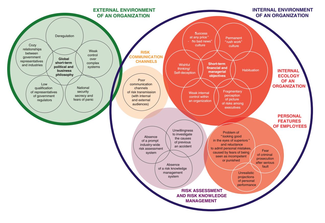
Chernov and Sornette’s model of the factors causing or contributing to risk concealment.
When summed up, many patterns of information concealment recur again and again. They sketch out a model of the causes of concealment, with about 20 causes grouped into five major clusters: the external environment enticing concealment, risk communication channels blocked, an internal ecology stimulating concealment or ignorance, faulty risk assessment and knowledge management, and people having personal incentives to conceal.
The problem is very much systemic: having just one or two of the causative problems can be counteracted by good risk management, but when several causes start to act together they become much harder to deal with – especially since many corrode the risk management ability of the entire organisation. Once risks are hidden, it becomes harder to manage them (management, after all, is done through information). Conversely, they list examples of successful risk information management: risk concealment may be something that naturally tends to emerge, but it can be counteracted.
Chernov and Sornette also apply their model to some technologies they think show signs of risk concealment: shale energy, GMOs, real debt and liabilities of the US and China, and the global cyber arms race. They are not arguing that a disaster is imminent, but the patterns of concealment are a reason for concern: if they persist, they have potential to make things worse the day something breaks.
Is information concealment the cause of all major disasters? Definitely not: some disasters are just due to exogenous shocks or surprise failures of technology. But as Fukushima shows, risk concealment can make preparation brittle and handling the aftermath inefficient. There is also likely plentiful risk concealment in situations that will never come to attention because there is no disaster necessitating and enabling a thorough investigation. There is little to suggest that the examined disasters were all uniquely bad from a concealment perspective.
From an information hazard perspective, this book is an important rejoinder: yes, some information is risky. But lack of information can be dangerous too. Many of the reasons for concealment like national security secrecy, fear of panic, prevention of whistle-blowing, and personnel being worried about personally being held accountable for a serious fault are maladaptive information hazard management strategies. The worker not reporting a mistake is handling a personal information hazard, at the expense of the safety of the entire organisation. Institutional secrecy is explicitly intended to contain information hazards, but tends to compartmentalize and block relevant information flows.
A proper information hazard management strategy needs to take the concealment risk into account too: there is a risk cost of not sharing information. How these two risks should be rationally traded against each other is an important question to investigate.

 distributed as
 ") . The goal of the watchlist is to spend expensive investigatory resources to figure out the true values; say the cost is 1 per item. Then a watchlist of randomly selected items will have a mean value
. The goal of the watchlist is to spend expensive investigatory resources to figure out the true values; say the cost is 1 per item. Then a watchlist of randomly selected items will have a mean value ![V=E[x]-1](http://s0.wp.com/latex.php?latex=V%3DE%5Bx%5D-1&bg=ffffff&fg=000000&s=0 "V=E[x]-1") . Suppose a cursory investigation costing much less gives some indication about
. Suppose a cursory investigation costing much less gives some indication about  . One approach is to select all items above a threshold
  , making
 ![V=E[x_i|y_i<\theta]-1](http://s0.wp.com/latex.php?latex=V%3DE%5Bx_i%7Cy_i%3C%5Ctheta%5D-1&bg=ffffff&fg=000000&s=0 "V=E[x_i|y_i<\theta]-1") .
., \epsilon \sim N(0,\sigma_\epsilon^2)") , then
, then  \Phi\left(\frac{t-\mu_x}{\sqrt{\sigma_x^2+\sigma_\epsilon^2}}\right)dt") . While one can ram through this using
. While one can ram through this using  (the correlation between x and y is 0.707, so this is not too much noise):
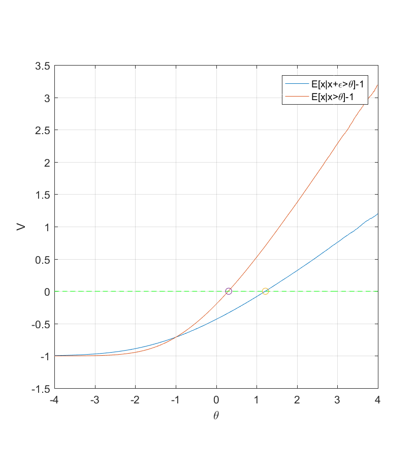
 data points and seen
  big surprises (remember that the first data point counts as one!), then the probability of a new surprise for your next data point is
  . So if you expect
  data points in total, when
 /N \ll 1") you can start to trust the estimates… assuming surprises are uncorrelated etc. Which you will not be certain about. The progression towards greater precision may be anything but dull.
you can start to trust the estimates… assuming surprises are uncorrelated etc. Which you will not be certain about. The progression towards greater precision may be anything but dull.
 , and the center of mass of the polyhedron is just the sum of the simplex centers of mass weighted by their volumes:
  . The volume of a simplex is
 \mathrm{det}(X_j)") where
where ![X_j=[x_{1j};x_{2j};\ldots;x_{Dj}]](http://s0.wp.com/latex.php?latex=X_j%3D%5Bx_%7B1j%7D%3Bx_%7B2j%7D%3B%5Cldots%3Bx_%7BDj%7D%5D&bg=ffffff&fg=000000&s=0 "X_j=[x_{1j};x_{2j};\ldots;x_{Dj}]") , the matrix made by sticking together the coordinate vectors of a simplex. Once we know this we can project the center of mass onto the plane of a face by finding its nullspace (the higher dimensional counterpart to a normal)
, the matrix made by sticking together the coordinate vectors of a simplex. Once we know this we can project the center of mass onto the plane of a face by finding its nullspace (the higher dimensional counterpart to a normal) \vec{n}") . Finally, to check whether the projection is inside the face, we can look at the matrix A where each column is the coordinates of one of the faces minus
. Finally, to check whether the projection is inside the face, we can look at the matrix A where each column is the coordinates of one of the faces minus  and the final row just ones, and solve for Ax=b where b is zero except for a one in the last row (
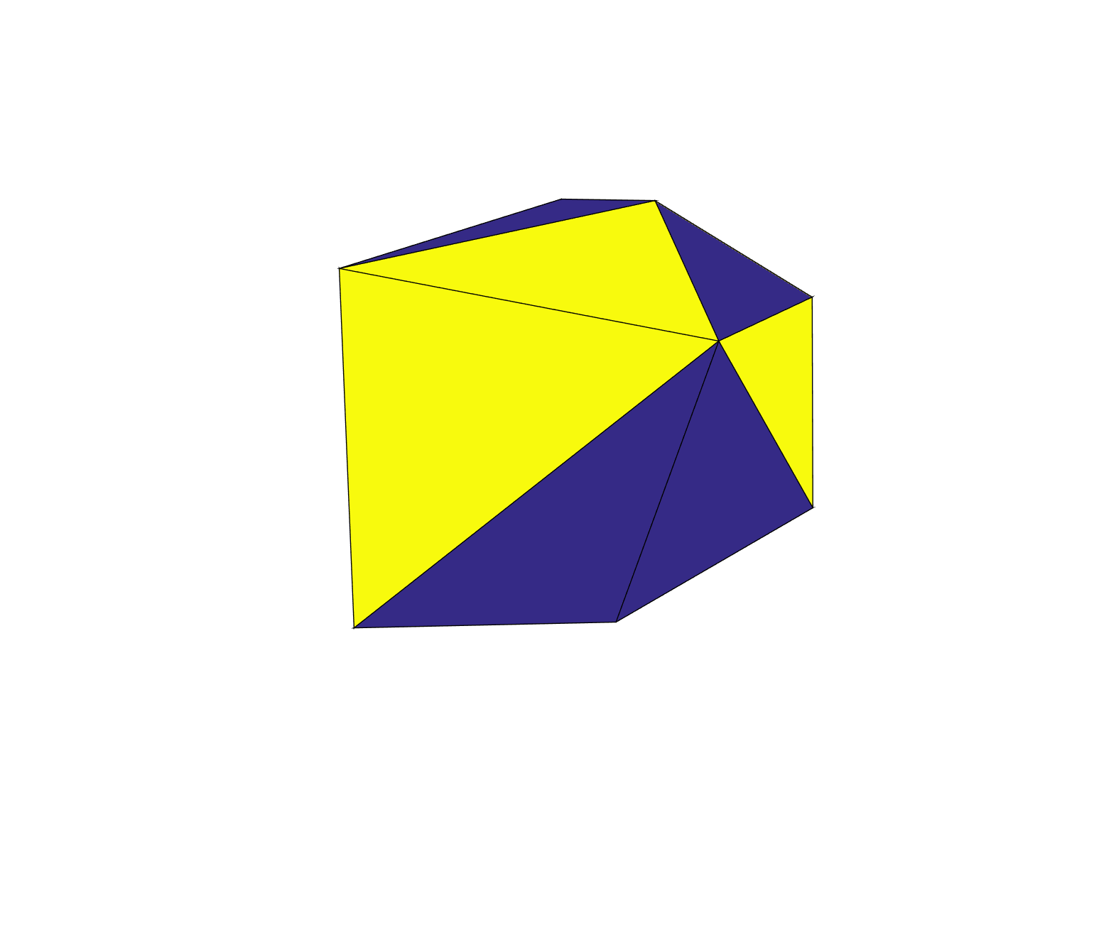

 ), but the number of stable faces also increases exponentially with D (as $latex 2^{0.9273 D}$).
D})=0.8407 D \ln(2) / \ln(D-1) \propto D/\ln(D)") . Even high-dimensional polytopes will stop flipping quickly in general. (A unistable polytope on the other hand can run through at least half of its faces, so there are some very slow ones too).
. Even high-dimensional polytopes will stop flipping quickly in general. (A unistable polytope on the other hand can run through at least half of its faces, so there are some very slow ones too). (if they were optimally distributed it would be
  ). At the same time, if N is relatively small compared to D (the polytope is simplex-like), the average diameter (the longest edge) of each face seems to approach
  . Why? I think this is because
 ") , the mean of a flipped k=2 Weibull distribution that shows up because of
, the mean of a flipped k=2 Weibull distribution that shows up because of  . Faces hence tends to be fairly wide unless N is large compared to D, but there will typically always be a few very narrow ones that are tricky to balance on.
") around the normal projection point (which is at distance d from the center of mass) where the vertical projection can intersect the face. Only parts of the hypersphere surface that are inside the face represent orientations that are stable. Even an unstable face can (sometimes) be stabilized if you turn it so that the tilted projection is inside, but for sufficiently high angles the hypersphere will be bigger than the face and it cannot be stable.
around the normal projection point (which is at distance d from the center of mass) where the vertical projection can intersect the face. Only parts of the hypersphere surface that are inside the face represent orientations that are stable. Even an unstable face can (sometimes) be stabilized if you turn it so that the tilted projection is inside, but for sufficiently high angles the hypersphere will be bigger than the face and it cannot be stable.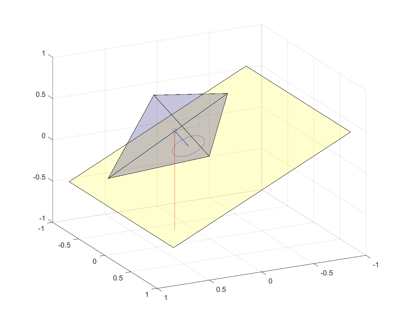
 the first condition might be tougher to meet than the second, but this is just a guess.