First, how do you make a Steiner chain? It is easy using inversion geometry. Just decide on the number of circles tangent to the inner circle (). Then the ratio of the radii of the inner and outer circle will be . The radii of the circles in the ring will be and their centres are located at distance from the origin. This produces a staid concentric arrangement. Now invert with relation to an arbitrary circle: all the circles are mapped to other circles, their tangencies preserved. Voila! A suitably eccentric Steiner chain to play with.
Since the original concentric chain obviously can be rotated continuously without losing touch with the inner and outer circle, this also generates a continuous family of circles after the inversion. This is why Steiner’s porism is true: if you can make the initial chain, you get an infinite number of other chains with the same number of circles.
Iterated function systems with circle maps
The fractal works by putting copies of the whole set of circles in the chain into each circle, recursively. I remap the circles so that the outer circle becomes the unit circle, and then it is easy to see that for a given small circle with (complex) centre and radius the map maps the interior of the unit circle to it. Use the ease of rotating the original concentric ring to produce an animation, and we can reconstruct the fractal.
Done.
Except… it feels a bit dry.
Ever since I first encountered iterated function systems in the 1980s I have felt they tend towards a geometric aesthetics that is not me, ferns notwithstanding. A lot has to do with the linearity of the transformations. One can of course add rotations, which cheers up the fractal a bit.
But still, I love the nonlinearity and harmony of conformal mappings.
Inversion makes things better!
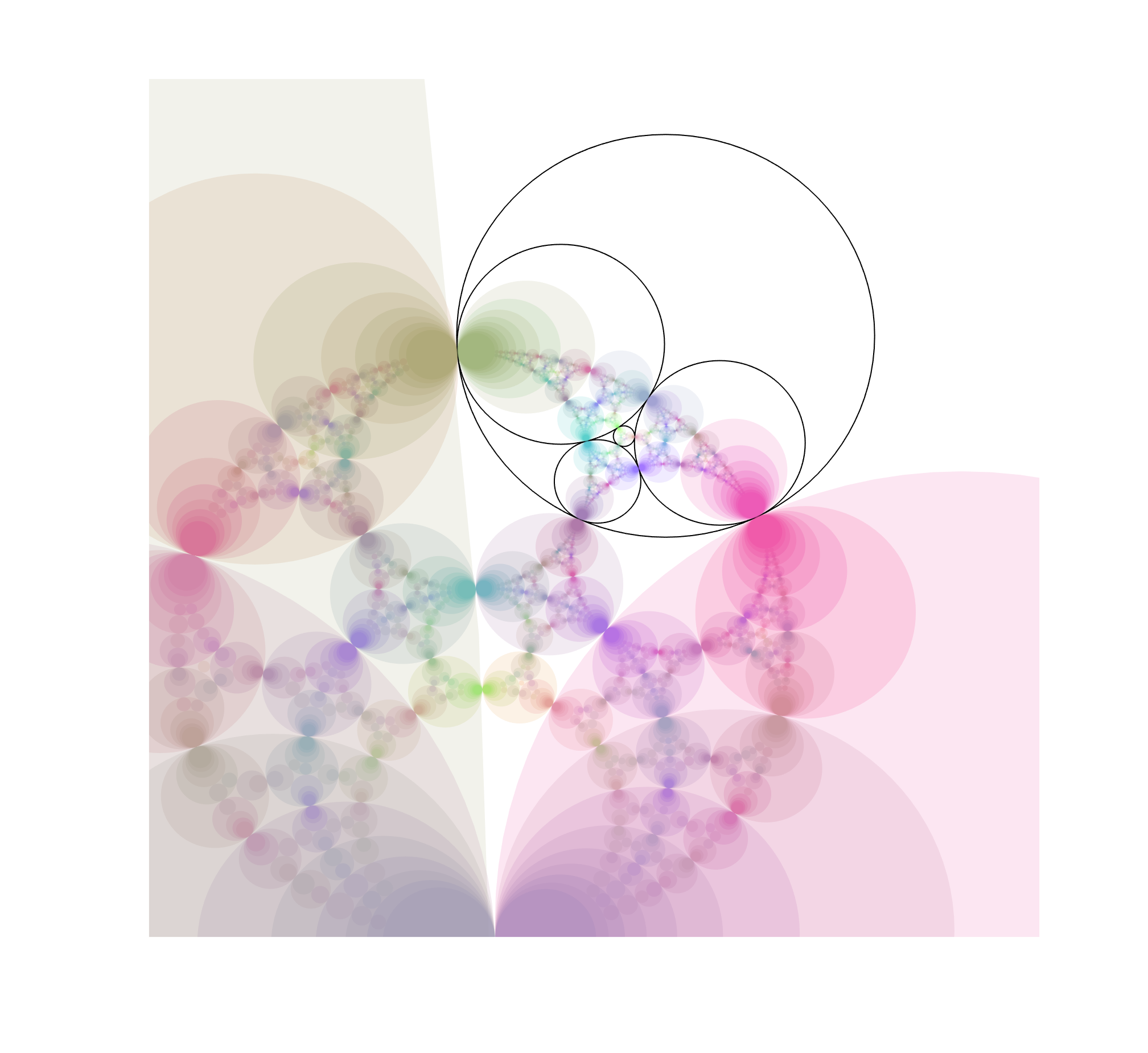
Enter the circle inversion fractals. They are the sets of the plane that map to themselves when being inverted in any and all of a set of generating circles (or, equivalently, the limit set of points under these inversions). As a rule of thumb, when the circles do not touch the fractal will be Cantor/Fatou-style fractal dust. When the circles are tangent the fractal will pass through the point of tangency. If three circles are tangent the fractal will contain a circle passing through these points. Since Steiner chains have lots of tangencies, we should get a lot of delicious fractals by using them as generators.
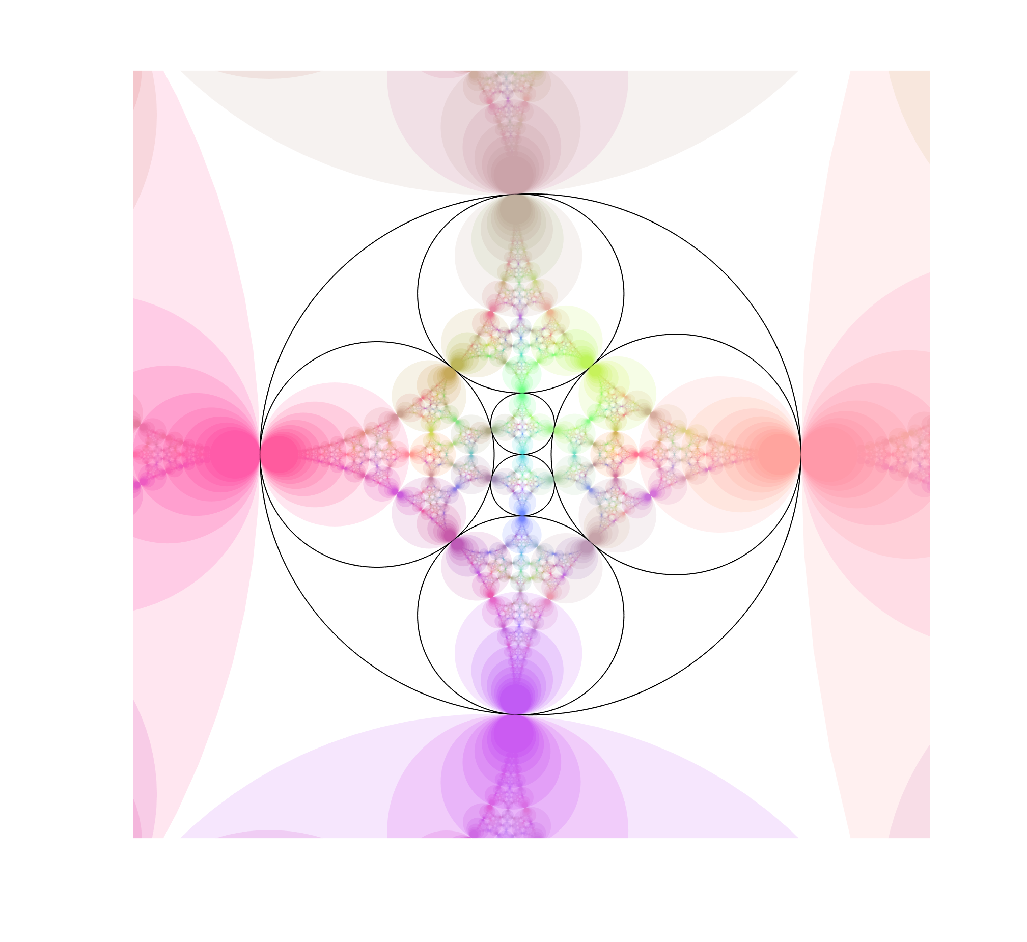
I use nearly the same code I used for the elliptic inversion fractals, mostly because I like the colours. The “real” fractal is hidden inside the nested circles, composed of an infinite Apollonian gasket of circles.
Note how the fractal extends outside the generators, forming a web of circles. Convergence is slow near tangent points, making it “fuzzy”. While it is easy to see the circles that belong to the invariant set that are empty, there are also circles going through the foci inside the coloured disks, touching the more obvious circles near those fuzzy tangent points. There is a lot going on here.
But we can complicate things by allowing the chain to slide and see how the fractal changes.
I recently returned to toying around with circle and sphere inversion fractals, that is, fractal sets that are invariant under inversion in a given set of circles or spheres.
That got me thinking: can you invert points in other things than circles? Of course you can! José L. Ramírez has written a nice overview of inversion in ellipses. Basically a point is projected to another point so that where is the centre of the ellipse and is the point where the ray between intersects the ellipse.
In Cartesian coordinates, for an ellipse centered on the origin and with semimajor and minor axes , the inverse point of is where and . Basically this is a squashed version of the circle formula.
Many of the properties remain the same. Lines passing through the centre of the ellipse are unchanged. Other lines get mapped to ellipses; if they intersect the inversion ellipse the new ellipse also intersect it at those points. Hence tangent lines are mapped to tangent ellipses. Ellipses with parallel axes and equal eccentricities map onto other ellipses (or lines if they intersect the centre of the inversion ellipse). Other conics get turned into cubics; for example a hyperbola gets mapped to a lemniscate. (See also this paper for more examples).
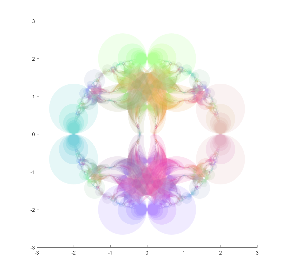
Now, from a fractal standpoint this means that if you have a set of ellipses that are tangent you should expect a fractal passing through their points of tangency. Basically all of the standard circle inversion fractals hence have elliptic counterparts. Here is the result for a ring of 4 or 6 mutually tangent ellipses:
Invariant set fractal (blue) for inversion in the red ellipses. Generated using an IFS algorithm.
These pictures were generated by taking points in the plane and inverting them with randomly selected ellipses; as the process continues they get attracted to the invariant set (this is basically a standard iterated function system). It also has the known problem of finding the points at the tangencies, since the iteration has to loop consistently between inverting in the two ellipses to get there, but it is likely that a third will be selected at some point.
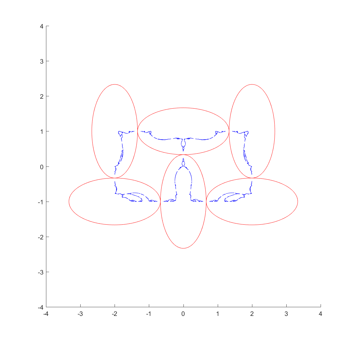
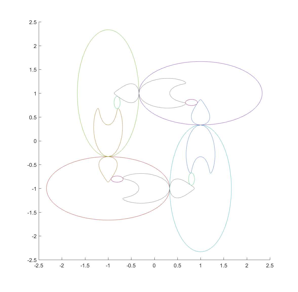
One approach is to deliberately recurse downward to find the points using a depth first search. We can take look at where each ellipse is mapped by each of the inversions, and since the fractal is inside each of the mapped ellipses we can then continue mapping the chain of mapped ellipses, getting nice bounds on where it is going (as long as everything is shrinking: this is guaranteed as long as it is mappings from the outside to the inside of the generating ellipses, but if they were to overlap things can explode). Doing this for just one step reveals one reason for the quirky shapes above: some of the ellipses get mapped into crescents or pears, adding a lot of bends:
Mappings of the ellipses by their inversions: each of the four main ellipses map the other three to their interior but distort the shape of two of them.
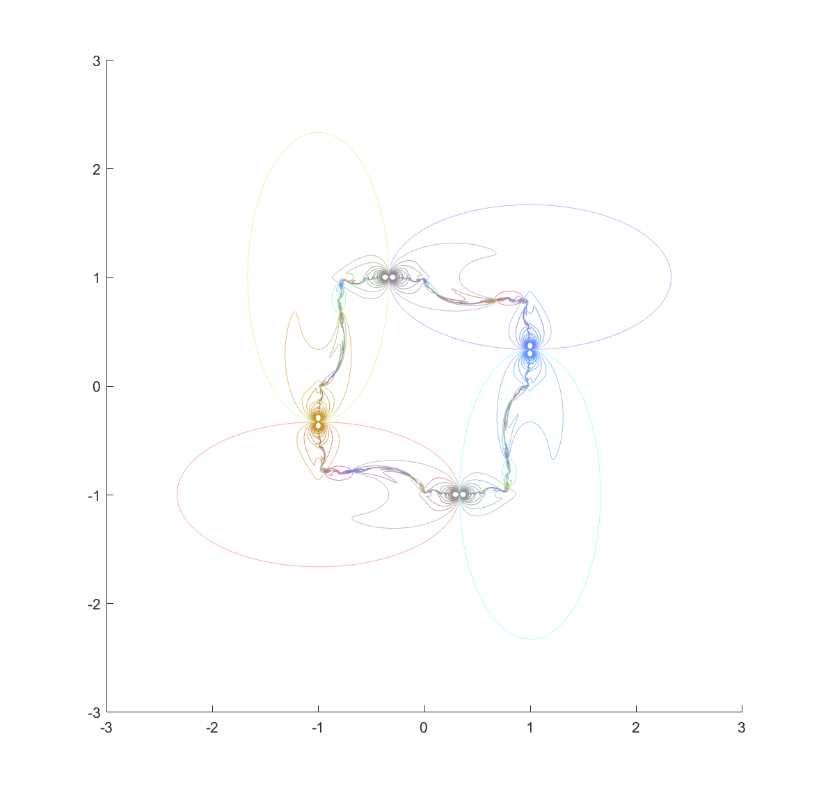
Now, continuing this process makes a nested structure where the invariant set is hidden inside all the other mapped ellipses.
Nested mappings of the ellipses in the chain, bounding the invariant set. Colors are mixtures of the colors of the generating ellipses, with an increase in saturation.
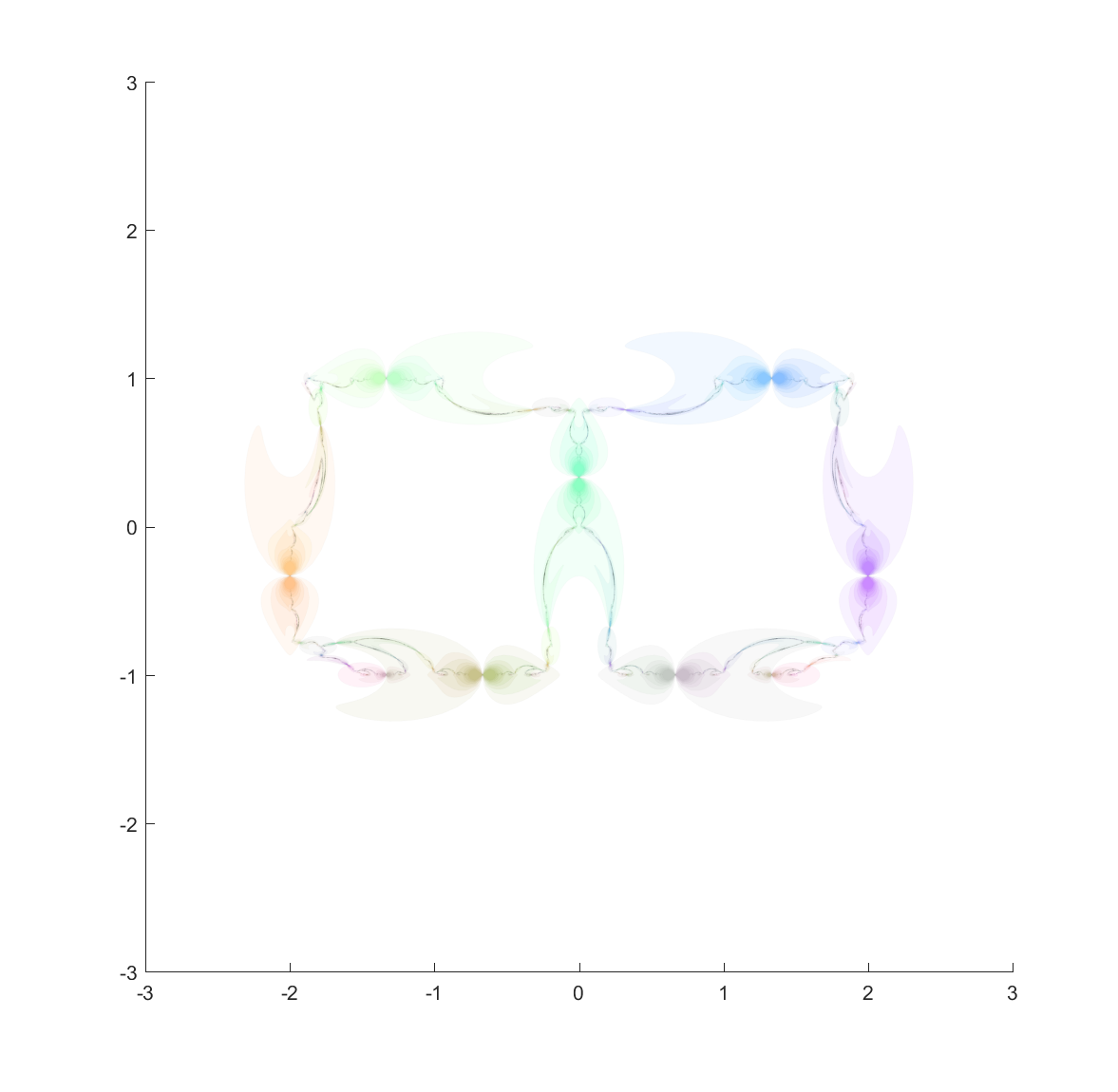
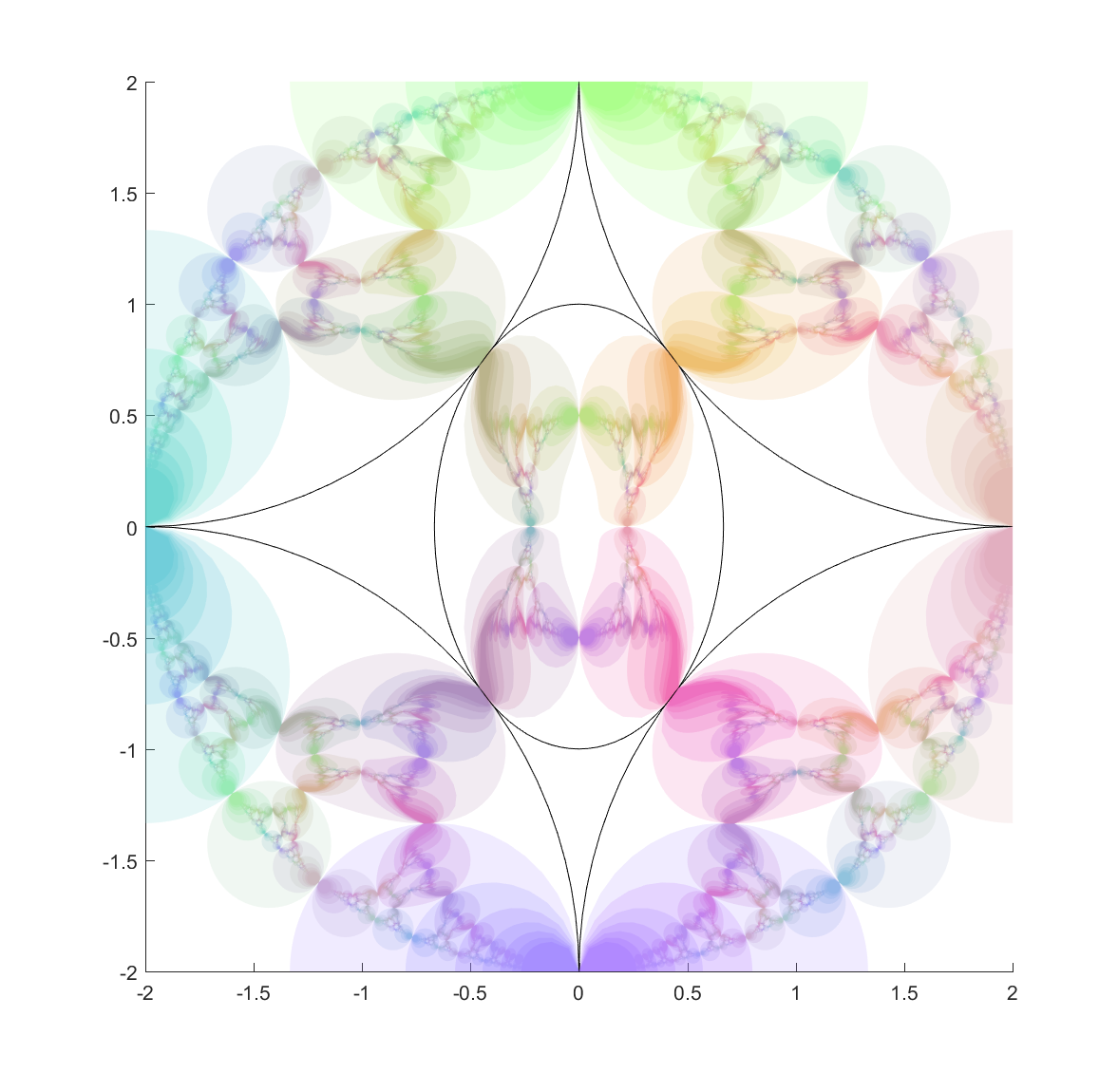
It is still hard to reach the tangent points, but at least now they are easier to detect. They are also numerically tough: most points on the ellipse circumferences are mapped away from them towards the interior of the generating ellipse. Still, if we view the mapped ellipses as uncertainties and shade them in we can get a very pleasing map of the invariant set:
Invariant set of chain of four outer ellipses and a circle tangent to them on the inside.
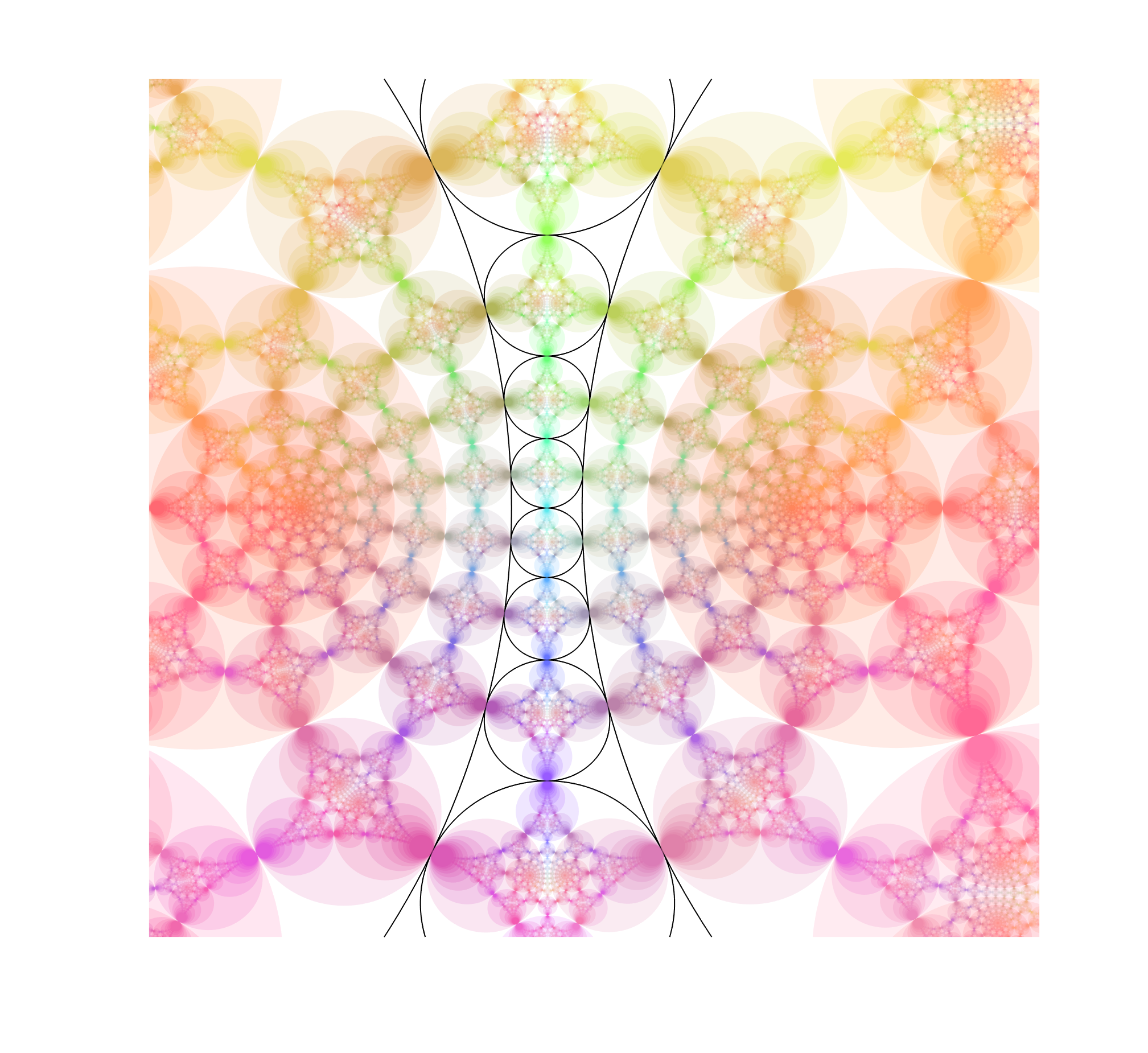
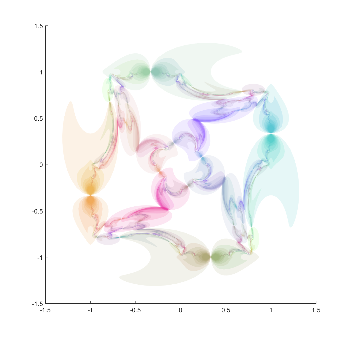
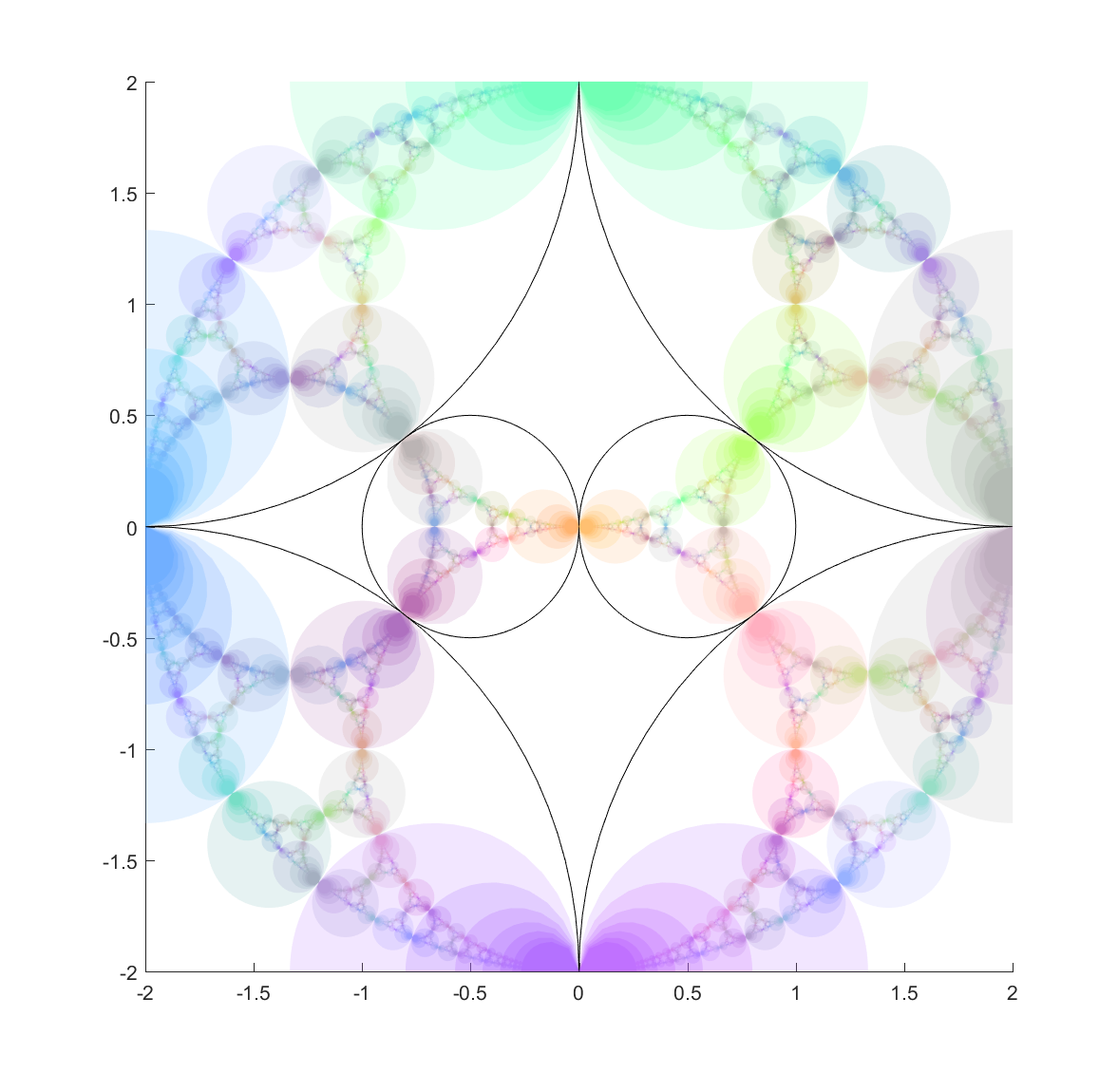
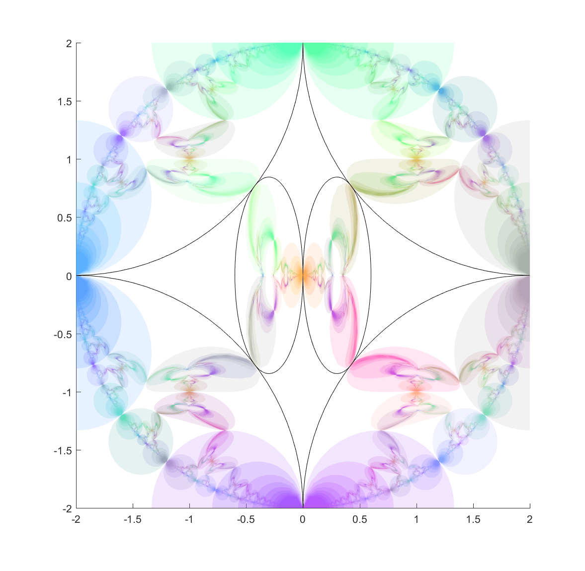
Here are a few other nice fractals based on these ideas:
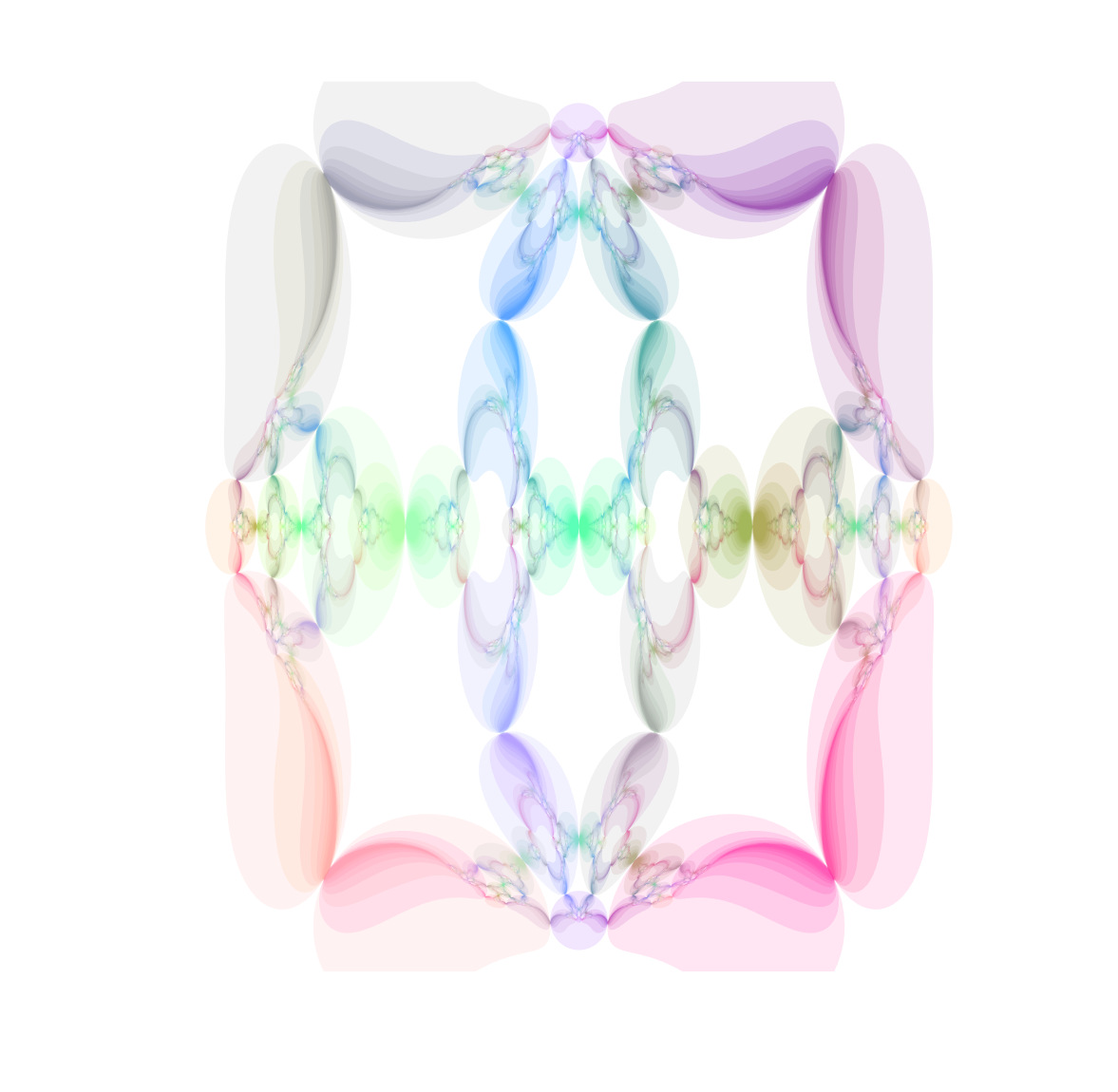
Using a mix of circles and ellipses produces a nice mix of the regularity of the circle-based Apollonian gaskets and the swooshy, Hénon fractal shape the ellipses induce.
function recurseDown(X,ellword,maxlevel,center)
i=ellword(end); % invert in latest ellipse
%
% Perform inversion
C=center(i,1:2);
A2=center(i,3).^2;
B2=center(i,4).^2;
Y(:,1)=X(:,1)-C(:,1);
Y(:,2)=X(:,2)-C(:,2);
X(:,1)=C(:,1)+A2.*B2.*Y(:,1)./(B2.*Y(:,1).^2+A2.*Y(:,2).^2);
X(:,2)=C(:,2)+A2.*B2.*Y(:,2)./(B2.*Y(:,1).^2+A2.*Y(:,2).^2);
%
if (norm(max(X)-min(X))<0.005) return; end
%
co=hsv(size(center,1));
coco=mean([1 1 1; 1 1 1; co(ellword,:)]);
%
%    plot(X(:,1),X(:,2),'Color',coco)
fill(X(:,1),X(:,2),coco,'FaceAlpha',.2,'EdgeAlpha',0)
%
if (length(ellword)<maxlevel)
    for j=1:size(center,1)
        if (j~=i)
            recurseDown(X,[ellword j],maxlevel,center)
        end
    end
end

)/(1+\sin(\pi/n))")
/2")
/2")


=(w+z)r")


 is projected to another point
  so that
  where
where  is the centre of the ellipse and
  is the point where the ray between
  intersects the ellipse.
 , the inverse point of
 ") is
is ") where
where  and
and  . Basically this is a squashed version of the circle formula.
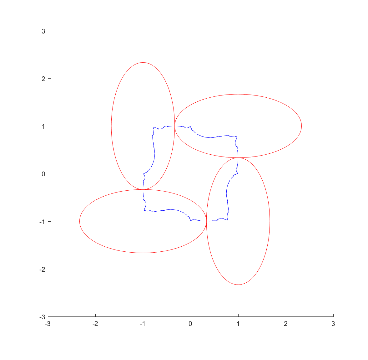