In a discussion Dennis Pamlin suggested that one could make a mortality table/survival curve for our species subject to existential risk, just as one can do for individuals. This also allows demonstrations of how changes in risk affect the expected future lifespan. This post is a small internal FHI paper I did just playing around with survivorship curves and other tools of survival analysis to see what they add to considerations of existential risk. The outcome was more qualitative than quantitative: I do not think we know enough to make a sensible mortality table. But it does tell us a few useful things:
- We should try to reduce ongoing “state risks” as early as possible
- Discrete “transition risks” that do not affect state risks matters less; we may want to put them off indefinitely.
- Indefinite survival is possible if we make hazard decrease fast enough.
Simple model
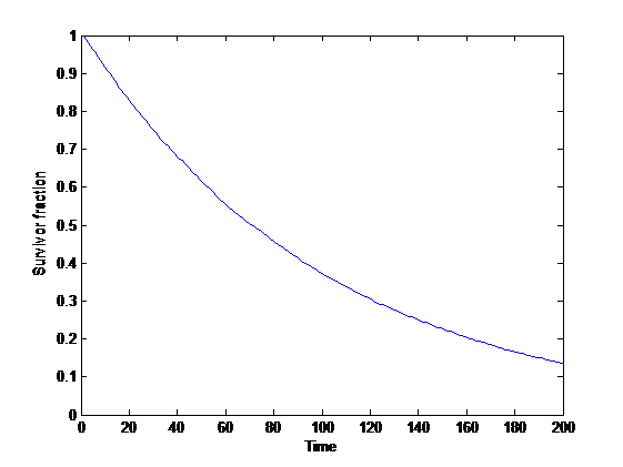
A first, very simple model: assume a fixed population and power-law sized disasters that randomly kill a number of people proportional to their size every unit of time (if there are survivors, then they repopulate until next timestep). Then the expected survival curve is an exponential decay.
This is in fact independent of the distribution, and just depends on the chance of exceedance. If disasters happen at a rate 
 = p")
 = \exp(-p \lambda t).")
This can be viewed as a simple model of state risks, the ongoing background of risk to our species from e.g. asteroids and supernovas.
Correlations
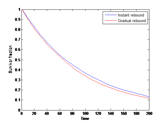
What if the population rebound is slower than the typical inter-disaster interval? During the rebound the population is more vulnerable to smaller disasters. However, if we average over longer time than the rebound time constant we end up with the same situation as before: an adjusted, slightly higher hazard, but still an exponential.
In ecology there has been a fair number of papers analyzing how correlated environmental noise affects extinction probability, generally concluding that correlated (“red”) noise is bad (e.g. (Ripa and Lundberg 1996), (Ovaskainen and Meerson 2010)) since the adverse conditions can be longer than the rebound time.
If events behave in a sufficiently correlated manner, then the basic survival curve may be misleading since it only shows the mean ensemble effect rather than the tail risks. Human societies are also highly path dependent over long timescales: our responses can create long memory effects, both positive and negative, and this can affect the risk autocorrelation.
Population growth
If population increases exponentially at a rate 
.")
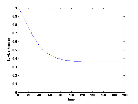
This is somewhat similar to Stuart’s and my paper on indefinite survival using backups: when we grow fast enough there is a finite chance of surviving indefinitely. The growth may be in terms of individuals (making humanity more resilient to larger and larger disasters), or in terms of independent groups (making humanity more resilient to disasters affecting a location). If risks change in size in proportion to population or occur in different locations in a correlated manner this basic analysis may not apply.
General cases
Overall, if there is a constant rate of risk, then we should expect exponential survival curves. If the rate grows or declines as a power 
^k.")
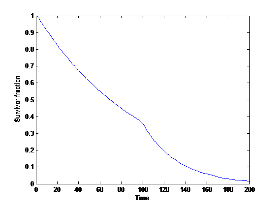
If we think of risk increasing from some original level to a new higher level, then the survival curve will essentially be piece-wise exponential with a more or less softly interpolating “knee”.
Transition risks
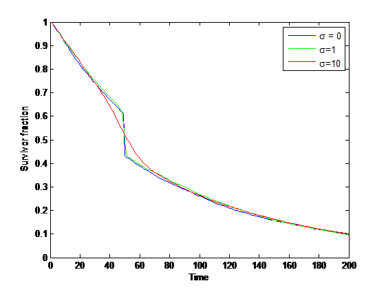
A transition risk is essentially an impulse of hazard. We can treat it as a Dirac delta function with some weight 

}{S(\mathrm{before }t)}=w")
Rectangular survival curves
Human individual survival curves are rectangularish because of exponentially increasing hazard plus some constant hazard (the Gompertz-Makeham law of mortality). The increasing hazard is due to ageing: old people are more vulnerable than young people.
Do we have any reason to believe a similar increasing hazard for humanity? Considering the invention of new dangerous technologies as adding more state risk we should expect at least enough of an increase to get a more convex shape of the survival curve in the present era, possibly with transition risk steps added in the future. This was counteracted by the exponential growth of human population until recently.
How do species survival curves look in nature?
There is “van Valen’s law of extinction” claiming the normal extinction rate remains constant at least within families, finding exponential survivorship curves (van Valen 1973). It is worth noting that the extinction rate is different for different ecological niches and types of organisms.
However, fits with Weibull distributions seem to work better for Cenozoic foraminifera than exponentials (Arnold, Parker and Hansard 1995), suggesting the probability of extinction increases with species age. The difference in shape is however relatively small (k≈1.2), making the probability increase from 0.08/Myr at 1 Myr to 0.17/Myr at 40 Myr. Other data hint at slightly slowing extinction rates for marine plankton (Cermeno 2011).
In practice there are problems associated with speciation and time-varying extinction rates, not to mention biased data (Pease 1988). In the end, the best we can say at present appears to be that natural species survival is roughly exponentially distributed.
Conclusions for xrisk research
Survival curves contain a lot of useful information. The median lifespan is easy to read off by checking the intersection with the 50% survival line. The life expectancy is the area under the curve.
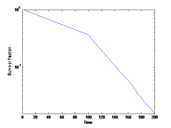
In a semilog-diagram an exponentially declining survival probability is a line with negative slope. The slope is set by the hazard rate. Changes in hazard rate makes the line a series of segments.
An early reduction in hazard (i.e. the line slope becomes flatter) clearly improves the outlook at a later time more than a later equal improvement: to have a better effect the late improvement needs to reduce hazard significantly more.
A transition risk causes a vertical displacement of the line (or curve) downwards: the weight determines the distance. From a given future time, it does not matter when the transition risk occurs as long as the subsequent hazard rate is not dependent on it. If the weight changes depending on when it occurs (hardware overhang, technology ordering, population) then the position does matter. If there is a risky transition that reduces state risk we should want it earlier if it does not become worse.
Acknowledgments
Thanks to Toby Ord for pointing out a mistake in an earlier version.
Appendix: survival analysis
The main object of interest is the survival function =\Pr(T>t)")

The event density =\frac{d}{dt}(1-S(t))")
The hazard function ")
 = - S'(t)/S(t)")
The expected future lifetime given survival to time 
}\int_{t_0}^\infty S(t)dt.")