KIC 8462852 (“Tabby’s Star”) continues to confuse. I blogged earlier about why I doubt it is a Dyson sphere. SETI observations in radio and optical has not produced any finds. Now there is evidence that it has dimmed over a century timespan, something hard to square with the comet explanation. Phil Plait over at Bad Astronomy has a nice overview of the headscratching.
However, he said something that I strongly disagree with:
Now, again, let me be clear. I am NOT saying aliens here. But, I’d be remiss if I didn’t note that this general fading is sort of what you’d expect if aliens were building a Dyson swarm. As they construct more of the panels orbiting the star, they block more of its light bit by bit, so a distant observer sees the star fade over time.
However, this doesn’t work well either. … Also, blocking that much of the star over a century would mean they’d have to be cranking out solar panels.
Basically, he is saying that a century timescale construction of a Dyson shell is unlikely. Now, since I have argued that we could make a Dyson shell in about 40 years, I disagree. I got into a Twitter debate with Karim Jebari (@KarimJebari) about this, where he also doubted what the natural timescale for Dyson construction is. So here is a slightly longer than Twitter message exposition of my model.
Lower bound
There is a strict lower bound set by how long it takes for the star to produce enough energy to overcome the binding energy of the source bodies (assuming one already have more than enough collector area). This is on the order of days for terrestrial planets, as per Robert Bradbury’s original calculations.
Basic model
Starting with a small system that builds more copies of itself, solar collectors and mining equipment, one can get exponential growth.
A simple way of reasoning: if you have an area ") of solar collectors, you will have energy
of solar collectors, you will have energy ") to play with, where
to play with, where  is the energy collected per square meter. This will be used to lift and transform matter into more collectors. If we assume this takes
  Joules per square meter on average, we get
  = (k/x)A(t)") , which makes is an exponential function with time constant
, which makes is an exponential function with time constant  . If a finished Dyson shell has area
  meters and we start with an initial plant of size
 ") (say on the order of a few hundred square meters), then the total time to completion is
(say on the order of a few hundred square meters), then the total time to completion is \ln(A_D/A(0))") seconds. The logarithmic factor is about 50.
seconds. The logarithmic factor is about 50.
If we assume  W and
W and  MJ/kg (see numerics below), then t=78 days.
This is very much in line with Robert’s original calculations. He pointed out that given the sun’s power output Earth could be theoretically disassembled in 22 days. In the above calculations the time constant (the time it takes to get 2.7 times as much area) is 37 hours. So for most of the 78 days there is just a small system expanding, not making a significant dent in the planet nor being very visible over interstellar distances; only in the later part of the period will it start to have radical impact.
The timescale is robust to the above assumptions: sun-like main sequence stars have luminosities within an order of magnitude of the sun (so can only change a factor of 10), using asteroid material (no gravitational binding cost) brings down by a factor of 10; if the material needs to be vaporized increases by less than a factor of 10; if a sizeable fraction of the matter is needed for mining/transport/building systems goes down proportionally; much thinner shells (see below) may give three orders of magnitude smaller (and hence bump into the hard bound above). So the conclusion is that for this model the natural timescale of terrestrial planetary disassembly into Dyson shells is on the order of months.
Digging into the practicalities of course shows that there are some other issues. Material needs to be transported into place (natural timescale about a year for a moving something 1 AU), the heating effects are going to be major on the planet being disassembled (lots of energy flow there, but of course just boiling it into space and capturing the condensing dust is a pretty good lifting method), the time it takes to convert 1 kg of undifferentiated matter into something useful places a limit of the mass flow per converting device, and so on. This is why our conservative estimate was 40 years for a Mercury-based shell: we assumed a pretty slow transport system.
Numerical values
Estimate for : assuming that each square meter shell has mass 1 kg, that the energy cost comes from the mean gravitational binding energy of Earth per kg of mass (37.5 MJ/kg), plus processing energy (on the order of 2.65 MJ/kg for heating and melting silicon). Note that using Earth slows things significantly.
I had a conversation with Eric Drexler today, where he pointed out that assuming 1 kg/square meter for the shell is arbitrary. There is a particular area density that is special: given that solar gravity and light pressure both decline with the square of the distance, there exists a particular density \approx 0.78") gram per square meter, which will just hang there neutrally. Heavier shells will need to orbit to remain where they are, lighter shells need cables or extra weight to not blow away. This might hence be a natural density for shells, making a factor 1282 smaller.
gram per square meter, which will just hang there neutrally. Heavier shells will need to orbit to remain where they are, lighter shells need cables or extra weight to not blow away. This might hence be a natural density for shells, making a factor 1282 smaller.
Linear growth does not work
I think the key implicit assumption in Plait’s thought above is that he imagines some kind of alien factory churning out shell. If it produces it at a constant rate  , then the time until it a has produced a finished Dyson shell with area square meters. That will take
  seconds.
Current solar cell factories produce on the order of a few hundred MW of solar cells per year; assuming each makes about 2 million square meters per year, we need 140 million billion years. Making a million factories merely brings things down to 140 billion years. To get a century scale dimming time,  square meters per second, about the area of the Atlantic ocean.
This feels absurd. Which is no good reason for discounting the possibility.
Automation makes the absurd normal
As we argued in our paper, the key assumptions are (1) things we can do can be automated, so that if there are more machines doing it (or doing it faster) there will be more done. (2) we have historically been good at doing things already occurring in nature. (3) self-replication and autonomous action occurs in nature. 2+3 suggests exponentially growing technologies are possible where a myriad entities work in parallel, and 1 suggests that this allows functions such as manufacturing to be scaled up as far as the growth goes. As Kardashev pointed out, there is no reason to think there is any particular size scale for the activities of a civilization except as set by resources and communication.
Incidentally, automation is also why cost overruns or lack of will may not matter so much for this kind of megascale projects. The reason Intel and AMD can reliably make billions of processors containing billions of transistors each is that everything is automated. Making the blueprint and fab pipeline is highly complex and requires an impressive degree of skill (this is where most overruns and delays happen), but once it is done production can just go on indefinitely. The same thing is true of Dyson-making replicators. The first one may be a tough problem that takes time to achieve, but once it is up and running it is autonomous and merely requires some degree of watching (make sure it only picks apart the planets you don’t want!) There is no requirement of continued interest in its operations to keep them going.
Likely growth rates
But is exponential growth limited mostly by energy the natural growth rate? As Karim and others have suggested, maybe the aliens are lazy or taking their time? Or, conversely, that multi century projects are unexpectedly long-term and hence rare.
Obviously projects could occur with any possible speed: if something can construct something in time X, it can in generally be done half as fast. And if you can construct something of size X, you can do half of it. But not every speed or boundary is natural. We do not answer the question of why a forest or the Great Barrier reef have the size they do by cost overruns stopping them, or that they will eventually grow to arbitrary size, but the growth rate is so small that it is imperceptible. The spread of a wildfire is largely set by physical factors, and a static wildfire will soon approach its maximum allowed speed since part of the fire that do not spread will be overtaken by parts that do. The same is true for species colonizing new ecological niches or businesses finding new markets. They can run slow, it is just that typically they seem to move as fast as they can.
Human economic growth has been on the order of 2% per year for very long historical periods. That implies a time constant \approx 50") years. This is a “stylized fact” that remained roughly true despite very different technologies, cultures, attempts at boosting it, etc. It seems to be “natural” for human economies. So were a Dyson shell built as a part of a human economy, we might expect it to be completed in 250 years.
years. This is a “stylized fact” that remained roughly true despite very different technologies, cultures, attempts at boosting it, etc. It seems to be “natural” for human economies. So were a Dyson shell built as a part of a human economy, we might expect it to be completed in 250 years.
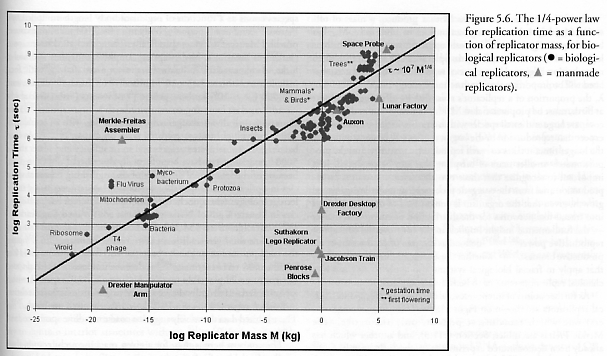
What about biological reproduction rates? Merkle and Freitas lists the replication time for various organisms and machines. They cover almost 25 orders of magnitude, but seem to roughly scale as  , where
  is the mass and
  . So if a total mass $M_T$ needs to be converted into replicators of mass , it will take time
 /\ln(2)") . Plugging in the first formula gives
. Plugging in the first formula gives /\ln(2)") . The smallest independent replicators have
. The smallest independent replicators have  (this gives
  minutes) while a big factory-like replicator (or a tree!) would have
  (
( years). In turn, if we set
  (a “light” Dyson shell) the time till construction ranges from 32 hours for the tiny to 378 years for the heavy replicator. Setting
  to an Earth mass gives a range from 36 hours to 408 years.
The lower end is infeasible, since this model assumes enough input material and energy – the explosive growth of bacteria-like replicators is not possible if there is not enough energy to lift matter out of gravity wells. But it is telling that the upper end of the range is merely multi-century. This makes a century dimming actually reasonable if we think we are seeing the last stages (remember, most of the construction time the star will be looking totally normal); however, as I argued in my previous post, the likelihood of seeing this period in a random star being englobed is rather low. So if you want to claim it takes millennia or more to build a Dyson shell, you need to assume replicators that are very large and heavy.
[Also note that some of the technological systems discussed in Merkle & Freitas are significantly faster than the main branch. Also, this discussion has talked about general replicators able to make all their parts: if subsystems specialize they can become significantly faster than more general constructors. Hence we have reason to think that the upper end is conservative.]
Conclusion
There is a lower limit on how fast a Dyson shell can be built, which is likely on the order of hours for manufacturing and a year of dispersion. Replicator sizes smaller than a hundred tons imply a construction time at most a few centuries. This range includes the effect of existing biological and economic growth rates. We hence have a good reason to think most Dyson construction is fast compared to astronomical time, and that catching a star being englobed is pretty unlikely.
I think that models involving slowly growing Dyson spheres require more motivation than models where they are closer to the limits of growth.
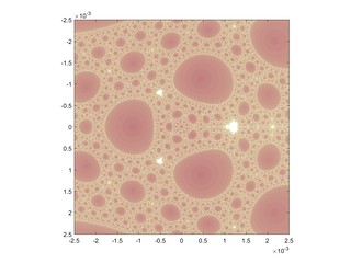
=z_n^2+c/z_n^3")


^{1/5}")


^{1/5}")
=0")
=z^2+c")

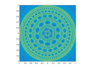

=\sum_{p \mathrm{is prime}} z^p") , the Taylor series that only includes all prime powers, combined with
, the Taylor series that only includes all prime powers, combined with =1") .
.
 (typically how many there are of some kind of object of size
  ), you formally define a function
 =\sum_{n=0}^\infty a_n z^n") , you derive some constraints on the function, and from this you get a formula for the
, you derive some constraints on the function, and from this you get a formula for the ") seriously as a (complex) function and use the powerful machinery of complex analysis to calculate asymptotic behavior for the
seriously as a (complex) function and use the powerful machinery of complex analysis to calculate asymptotic behavior for the 
 , while single tuck tie knots grow as
  .
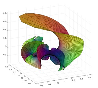
.=\sum_{n=0}^\infty X_n z^n") where
where  are independent random numbers, what kind of functions do we get? Trying it with complex Gaussian
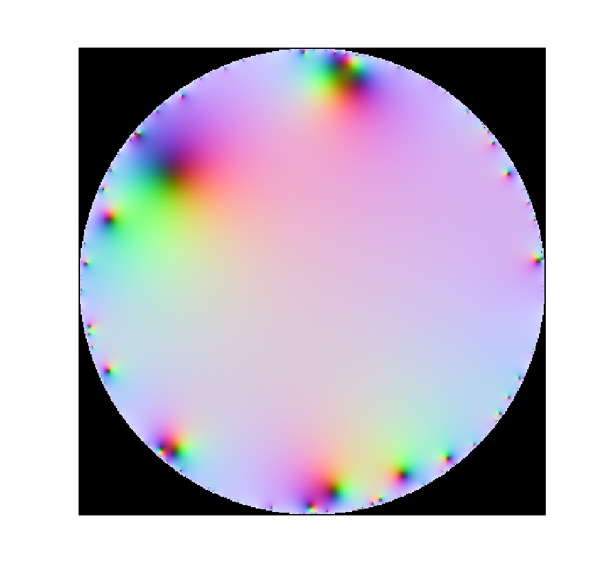
 we have an exponentially decaying sequence of
  , so if the
 ") and not too divergent variance we should expect convergence, while outside the unit circle any nonzero
and not too divergent variance we should expect convergence, while outside the unit circle any nonzero  \leq E(X)/t") to argue that a series
to argue that a series ") would converge if
would converge if /n") converges. However, this is not correct enough for proper mathematics. One entirely possible Gaussian outcome is
converges. However, this is not correct enough for proper mathematics. One entirely possible Gaussian outcome is  or worse. We need to speak of probabilistic convergence.
 of an uncontinuable function). In fact,
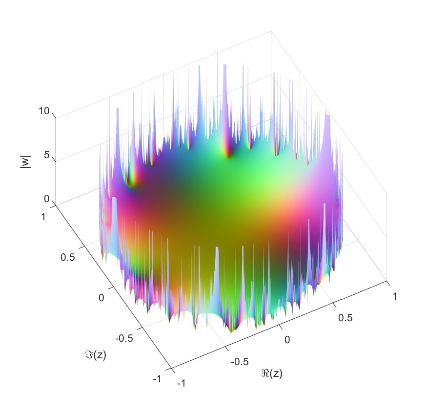


