Robin Hanson mentions that some people take him to task for working on one scenario (WBE) that might not be the most likely future scenario (“standard AI”); he responds by noting that there are perhaps 100 times more people working on standard AI than WBE scenarios, yet the probability of AI is likely not a hundred times higher than WBE. He also notes that there is a tendency for thinkers to clump onto a few popular scenarios or issues. However:
In addition, due to diminishing returns, intellectual attention to future scenarios should probably be spread out more evenly than are probabilities. The first efforts to study each scenario can pick the low hanging fruit to make faster progress. In contrast, after many have worked on a scenario for a while there is less value to be gained from the next marginal effort on that scenario.
This is very similar to my own thinking about research effort. Should we focus on things that are likely to pan out, or explore a lot of possibilities just in case one of the less obvious cases happens? Given that early progress is quick and easy, we can often get a noticeable fraction of whatever utility the topic has by just a quick dip. The effective altruist heuristic of looking at neglected fields also is based on this intuition.
A model
But under what conditions does this actually work? Here is a simple model:
There are 


Here is what happens if we allocate proportional to a power of the scenarios, 

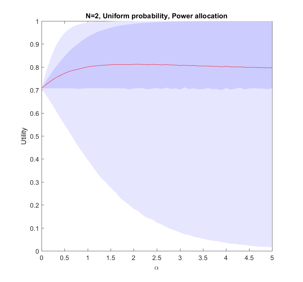
This is the 


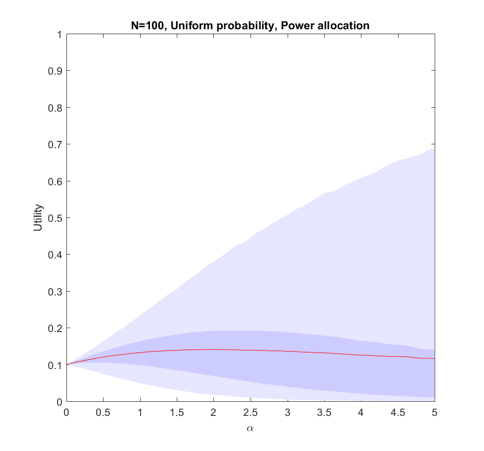
The 
What is going on?
This doesn’t seem to fit Robin’s or my intuitions at all! The best we can say about uniform allocation is that it doesn’t produce much regret: whatever happens, we will have made some allocation to the possibility. For large N this actually works out better than the directed allocation for a sizable fraction of realizations, but on average we get less utility than betting on the likely choices.
The problem with the model is of course that we actually know the probabilities before making the allocation. In reality, we do not know the likelihood of AI, WBE or alien invasions. We have some information, and we do have priors (like Robin’s view that 
We know nothing
Let us start by looking at the worst possible case: we do not know what the true probabilities are at all. We can draw estimates from the same distribution – it is just that they are uncorrelated with the true situation, so they are just noise.

In this case uniform distribution of effort is optimal. Not only does it avoid regret, it has a higher expected utility than trying to focus on a few scenarios (
Note that if we have to allocate a minimum effort to each investigated scenario we will be forced to effectively increase our
We know a bit
We can imagine that knowing more should allow us to gradually interpolate between the different results: the more you know, the more you should focus on the likely scenarios.
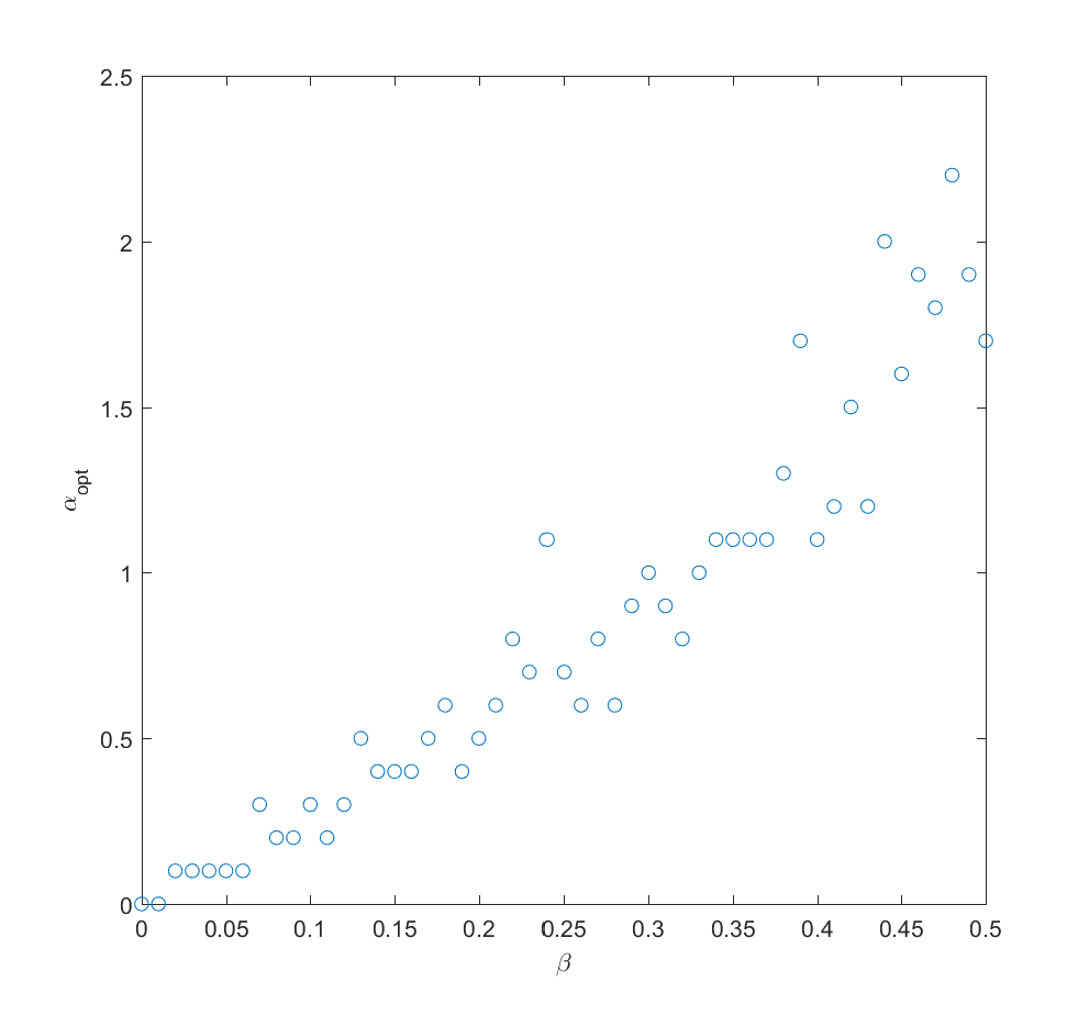
If we take the mean of the true probabilities with some randomly drawn probabilities (the “half random” case) the curve looks quite similar to the case where we actually know the probabilities: we get a maximum for 

Q_i)^\alpha")


We learn
Adding a bit of realism, we can consider a learning process: after allocating some effort 


=\sqrt{\gamma/N}/C")

=\sqrt{2\gamma/NC^2}")

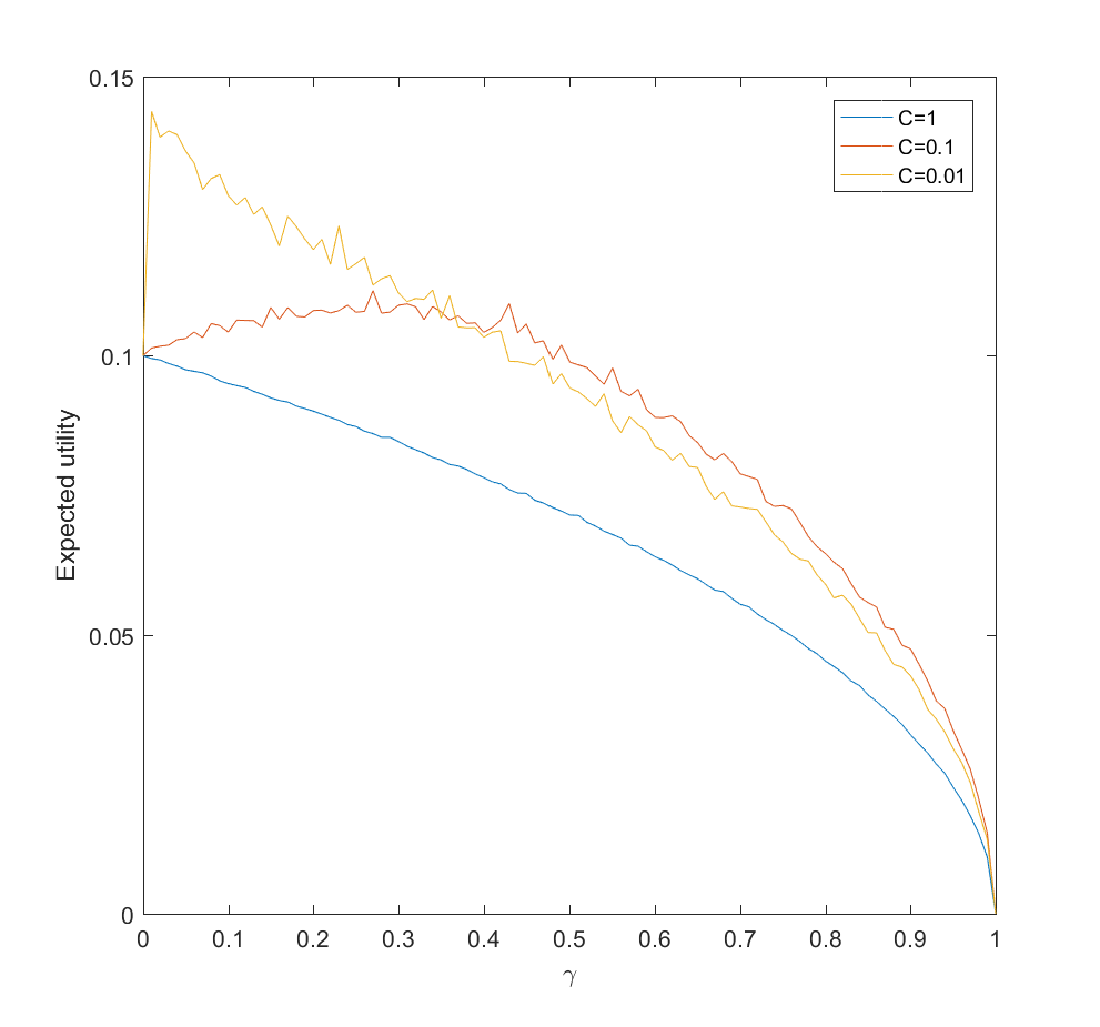
This is surprisingly inefficient. The reason is that the expected utility declines as 

Conclusions
So, how should we focus? These results suggest that the key issue is knowing how little we know compared to what can be known, and how much effort it would take to know significantly more.
If there is little more that can be discovered about what scenarios are likely, because our state of knowledge is pretty good, the world is very random, or improving knowledge about what will happen will be costly, then we should roll with it and distribute effort either among likely scenarios (when we know them) or spread efforts widely (when we are in ignorance).
If we can acquire significant information about the probabilities of scenarios, then we should do it – but not overdo it. If it is very easy to get information we need to just expend some modest effort and then use the rest to flesh out our scenarios. If it is doable but costly, then we may spend a fair bit of our budget on it. But if it is hard, it is better to go directly on the object level scenario analysis as above. We should not expect the improvement to be enormous.
Here I have used a square root diminishing return model. That drives some of the flatness of the optima: had I used a logarithm function things would have been even flatter, while if the returns diminish more mildly the gains of optimal effort allocation would have been more noticeable. Clearly, understanding the diminishing returns, number of alternatives, and cost of learning probabilities better matters for setting your strategy.
In the case of future studies we know the number of scenarios are very large. We know that the returns to forecasting efforts are strongly diminishing for most kinds of forecasts. We know that extra efforts in reducing uncertainty about scenario probabilities in e.g. climate models also have strongly diminishing returns. Together this suggests that Robin is right, and it is rational to stop clustering too hard on favorite scenarios. Insofar we learn something useful from considering scenarios we should explore as many as feasible.
> “(like Robin’s view that P_{WBE} > 100 P_{AI})”
I think you mean “P_{AI} < 100 P_{WBE}"?
(Assuming the above corresponds to the claim you quote in the opening paragraph – "the probability of AI is not a hundred times higher than WBE" – and not a different estimate of his about WBE's superior likelihood.)
Yes. I feel stupid. I think I should have learned the direction of inequality signs by now. Will fix. Thanks!
Would be really great to get some sort of dataset on just how fast insight diminishes with effort into scenarios. Probably are already some results on this for games like Chess or Go.
Agreed. I think there are a few done in forecasting studies; I think Scott Armstrong has a few stylized facts here. Will look into it.