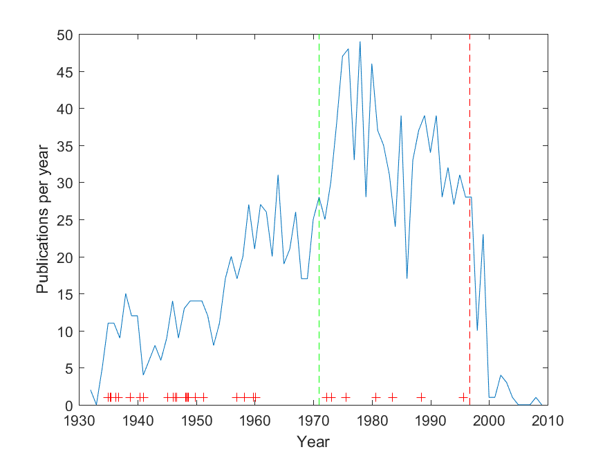
During my work on the Paris talk I began to wonder whether Paul Erdős (who I used as an example of a respected academic who used cognitive enhancers) could actually have been shown to have benefited from his amphetamine use, which began in 1971 according to Hill (2004). One way of investigating is his publication record: how many papers did he produce per year before or after 1971? Here is a plot, based on Jerrold Grossman’s 2010 bibliography:
Productivity of Paul Erdos over his life. Green dashed line: amphetamine use, red dashed line: death. Crosses mark named concepts.
The green dashed line is the start of amphetamine use, and the red dashed life is the date of death. Yes, there is a fairly significant posthumous tail: old mathematicians never die, they just asymptote towards zero. Overall, the later part is more productive per year than the early part (before 1971 the mean and standard deviation was 14.6±7.5, after 24.4±16.1; a Kruskal-Wallis test rejects that they are the same distribution, p=2.2e-10).
This does not prove anything. After all, his academic network was growing and he moved from topic to topic, so we cannot prove any causal effect of the amphetamine: for all we know, it might have been holding him back.
One possible argument might be that he did not do his best work on amphetamine. To check this, I took the Wikipedia article that lists things named after Erdős, and tried to find years for the discovery/conjecture. These are marked with red crosses in the diagram, slightly jittered. We can see a few clusters that may correspond to creative periods: one in 35-41, one in 46-51, one in 56-60. After 1970 the distribution was more even and sparse. 76% of the most famous results were done before 1971; given that this is 60% of the entire career it does not look that unlikely to be due to chance (a binomial test gives p=0.06).
Again this does not prove anything. Maybe mathematics really is a young man’s game, and we should expect key results early. There may also have been more time to recognize and name results from the earlier career.
In the end, this is merely a statistical anecdote. It does show that one can be a productive, well-renowned (if eccentric) academic while on enhancers for a long time. But given the N=1, firm conclusions or advice are hard to draw.
Erdős’s friends worried about his drug use, and in 1979 Graham bet Erdős $500 that he couldn’t stop taking amphetamines for a month. Erdős accepted, and went cold turkey for a complete month. Erdős’s comment at the end of the month was “You’ve showed me I’m not an addict. But I didn’t get any work done. I’d get up in the morning and stare at a blank piece of paper. I’d have no ideas, just like an ordinary person. You’ve set mathematics back a month.” He then immediately started taking amphetamines again. (Hill 2004)
One of the first fractals I ever saw was the Apollonian gasket, the shape that emerges if you draw the circle internally tangent to three other tangent circles. It is somewhat similar to the Sierpinski triangle, but has a more organic flair. I can still remember opening my copy of Mandelbrot’s The Fractal Geometry of Nature and encountering this amazing shape. There is a lot of interesting things going on here.
Here is a simple algorithm for generating related circle packings, trading recursion for flexibility:
Start with a domain and calculate the distance to the border for all interior points.
Place a circle of radius at the point with maximal distance from the border.
Recalculate the distances, treating the new circle as a part of the border.
Repeat (2-3) until the radius becomes smaller than some tolerance.
This is easily implemented in Matlab if we discretize the domain and use an array of distances , which is then updated where is the distance to the circle. This trades exactness for some discretization error, but it can easily handle nearly arbitrary shapes.
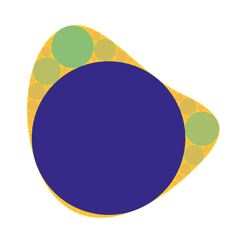
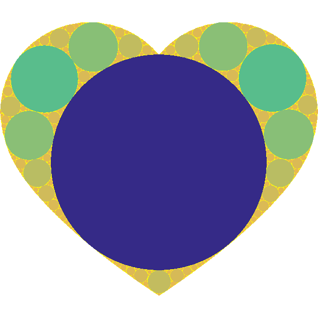
Apollonian circle packing in square.Apollonian circle packing in blob.Apollonian circle packing in heart.
It is interesting to note that the topology is Apollonian nearly everywhere: as soon as three circles form a curvilinear triangle the interior will be a standard gasket if .
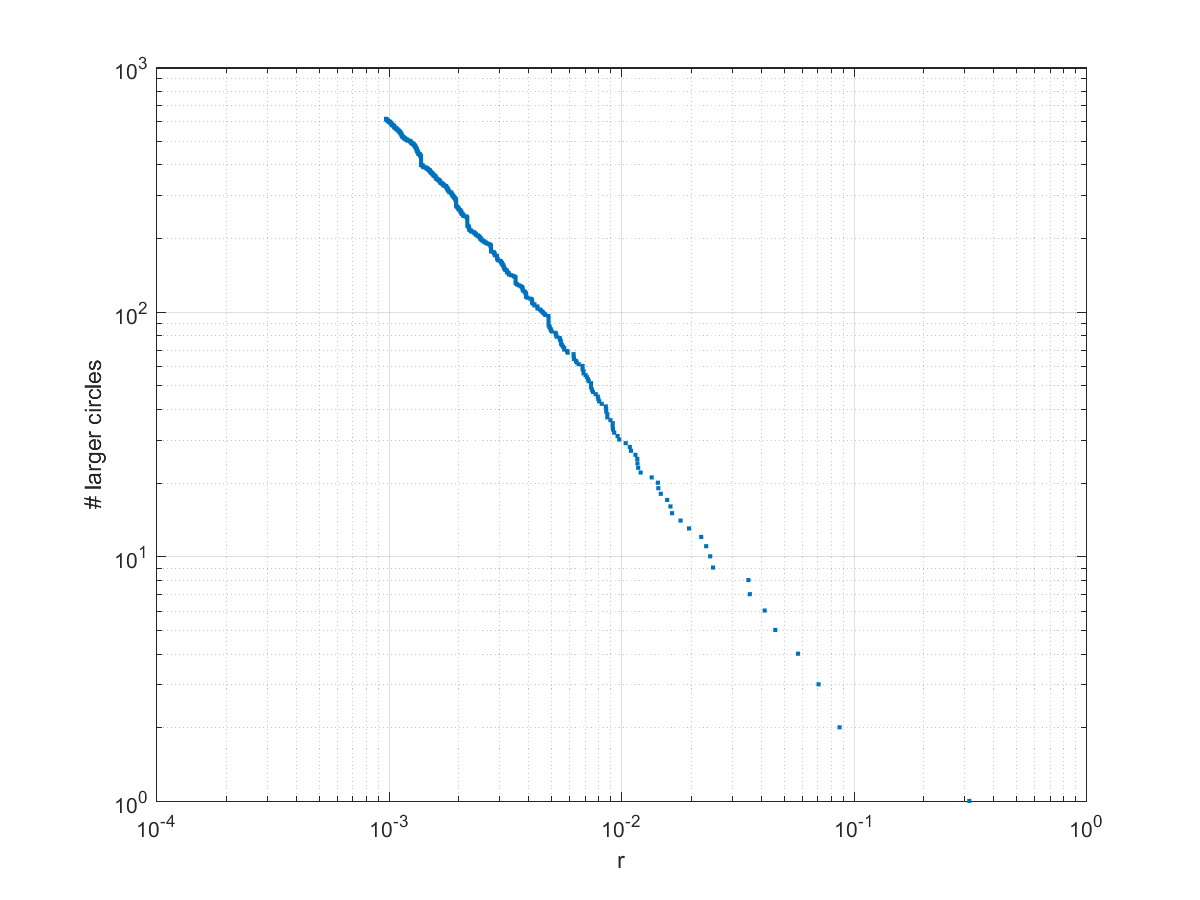
Number of circles larger than a certain radius in packing in blob shape.
In the above pictures the first circle tends to dominate. In fact, the size distribution of circles is a power law: the number of circles larger than r grows as as we approach zero, with . This is unsurprising: given a generic curved triangle, the inscribed circle will be a fraction of the radii of the bordering circles. If one looks at integral circle packings it is possible to see that the curvatures of subsequent circles grow quadratically along each “horn”, but different “horns” have different growths. Because of the curvature the self-similarity is nontrivial: there is actually, as far as I know, still no analytic expression of the fractal dimension of the gasket. Still, one can show that the packing exponent is the Hausdorff dimension of the gasket.
Anyway, to make the first circle less dominant we can either place a non-optimal circle somewhere, or use lower .
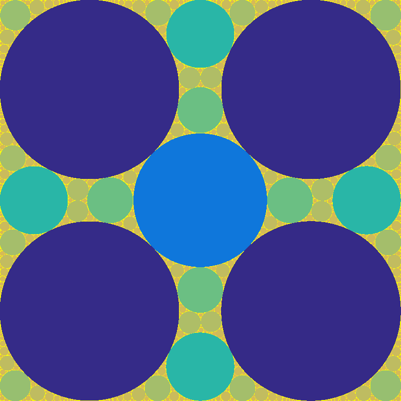
Apollonian packing in square with central circle of radius 1/6.
If we place a circle in the centre of a square with a radius smaller than the distance to the edge, it gets surrounded by larger circles.
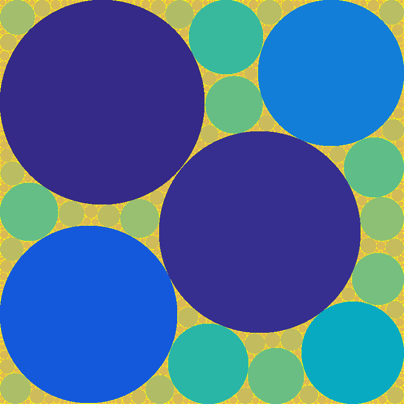
Randomly started Apollonian packing.
If the circle is misaligned, it is no problem for the tiling: any discrepancy can be filled with sufficiently small circles. There is however room for arbitrariness: when a bow-tie-shaped region shows up there are often two possible ways of placing a maximal circle in it, and whichever gets selected breaks the symmetry, typically producing more arbitrary bow-ties. For “neat” arrangements with the right relationships between circle curvatures and positions this does not happen (they have circle chains corresponding to various integer curvature relationships), but the generic case is a mess. If we move the seed circle around, the rest of the arrangement both show random jitter and occasional large-scale reorganizations.
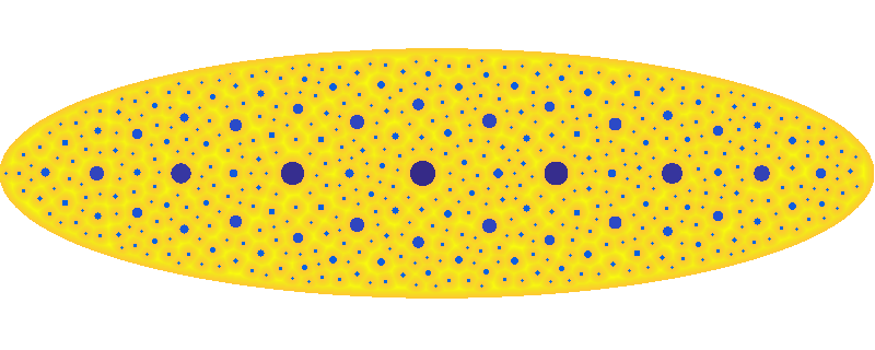
When we let we get sponge-like fractals: these are relatives to the Menger sponge and the Cantor set. The domain gets an infinity of circles punched out of itself, with a total area approaching the area of the domain, so the total measure goes to zero.
Apollonian packing with alpha=0.5.
That these images have an organic look is not surprising. Vascular systems likely grow by finding the locations furthest away from existing vascularization, then filling in the gaps recursively (OK, things are a bit more complex).
Apollonian packing with alpha=1/4.Apollonian packing with alpha=0.1.
What about nested/continued integrals? Here is a simple one:
.
The way to see this is to recognize that the x in the first integral is going to integrate to , the x in the second will be integrated twice , and so on.
In general additive integrals of this kind turn into sums (assuming convergence, handwave, handwave…):
.
On the other hand, .
So if we insert we get the sum . For we end up with . The differential equation has solution . Setting the integral is clearly zero, so . Tying it together we get:
.
Things are trickier when the integrals are multiplicative, like . However, we can turn it into a differential equation: which has the well known solution . Same thing for , giving us . Since we are running indefinite integrals we get those pesky constants.
Plugging in gives . If we set we get the mildly amusing and in retrospect obvious formula
.
We can of course mess things up further, like , where the differential equation becomes with the solution . A surprisingly simple solution to a weird-looking integral. In a similar vein:
(that is, you get an implicit but well defined expression for the (x,I(x)) values. With Lambert, the x and y axes always tend to switch place).
[And yes, convergence is handwavy in this essay. I think the best way of approaching it is to view the values of these integrals as the functions invariant under the functional consisting of the integral and its repeated function: whether nearby functions are attracted to it (or not) under repeated application of the functional depends on the case. ]
The gamma function has a long and interesting history (check out (Davis 1963) excellent review), but one application does not seem to have shown up: minimal surfaces.
A minimal surface is one where the average curvature is always zero; it bends equally in two opposite directions. This is equivalent to having the (locally) minimal area given its boundary: such surfaces are commonly seen as soap films stretched from frames. There exists a rich theory for them, linking them to complex analysis through the Enneper-Weierstrass representation: if you have a meromorphic function g and an analytic function f such that is holomorphic, then
produces a minimal surface .
When plugging in the hyperbolic tangent as g and using f=1 I got a new and rather nifty surface a few years back. What about plugging in the gamma function? Let .
We integrate from the regular point to different points in the complex plane. Let us start with the simple case of .
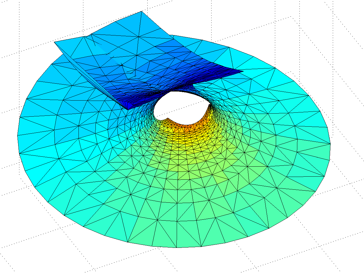
Gamma function minimal surface for z in 0.5<Re(z)<3.5, -8<Im(z)
The surface is a billowing strip, and as we include z with larger and larger real parts the amplitude of the oscillations grow rapidly, making it self-intersect. The behaviour is somewhat similar to the Catalan minimal surface, except that we only get one period. If we go to larger imaginary parts the surface approaches a horizontal plane. OK, the surface is a plane with some wild waves, right?
Not so fast, we have not looked at the mess for Re(z)<0. First, let’s examine the area around the z=0 singularity. Since the values of the integrand blows up close to it, they produce a surface expanding towards infinity – very similar to a catenoid. Indeed, catenoid ends tend to show up where there are poles. But this one doesn’t close exactly: for re(z)<0 there is some overshoot producing a self-intersecting plane-like strip.
Gamma function minimal surface close to the z=0 singularity. Colour denotes Re(z). Integration contours from 1 to z run clockwise for Im(z)<0 and counterclockwise for Im(z)>0.
The problem is of course the singularity: when integrating in the complex plane we need to avoid them, and depending on the direction we go around them we can get a complex phase that gives us an entirely different value of the function. In this case the branch cut corresponds to the real line: integrating clockwise or counter-clockwise around z=0 to the same z gives different values. In fact, a clockwise turn adds [3.6268i, 3.6268, 6.2832i] (which looks like – a rather neat residue!) to the coordinates: a translation in the positive y-direction. If we extend the surface by going an extra turn clockwise or counterclockwise a number of times, we get copies that attach seamlessly.
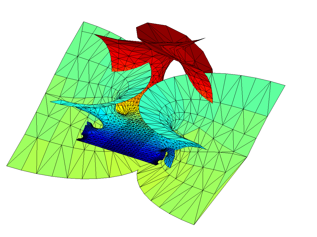
Gamma minimal surface extended by integration paths between the -1 and 0 singularities (blue patches).
Gamma minimal surface patch that can be repeated by translation along the y-axis. Colour denotes Re(z).
OK, we have a surface with some planar strips that turn wobbly and self-intersecting in the x-direction, with elliptic catenoid ends repeating along the y-direction due to the z=0 singularity. Going down the negative x-direction things look plane between the catenoids… except of course for the catenoids due to all the other singularities for . They also introduce residues along the y-direction, but different ones from the z=0 – their extensions of the surface will be out of phase with each other, making the fully extended surface fantastically self-intersecting and confusing.
Gamma function minimal surface extended by integrating around poles.
So, I think we have a simple answer to why the gamma function minimal surface is not well known: it is simply too messy and self-intersecting.
Of course, there may be related nifty surfaces. is nicely behaved and looks very much like the Enneper surface near zero, with “wings” that oscillate ever more wildly as we move towards the negative reals. No doubt there are other beautiful things to look for in the vicinity.
Another of my favourite functions if the Gamma function, , the continuous generalization of the factorial. While it grows rapidly for positive reals, it has fun poles for the negative integers and is generally complex. What happens when you iterate it?
First I started by just applying it to different starting points, . The result is a nice fractal, with some domains approaching 1, and others running off to infinity.
Here I color points that go to infinity in green shades on the number of iterations before they become very large, and the points approaching 1 by . Zooming in a bit more reveals neat self-similar patterns with alternating “beans”:
In the outside regions we have thin tendrils stretching towards infinity. These are familiar to anybody who has been iterating exponentials or trigonometric functions: the combination of oscillation and (super)exponential growth leads to the pattern.
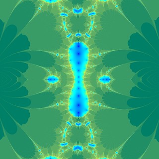
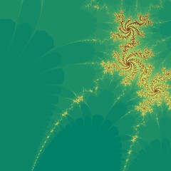
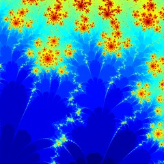
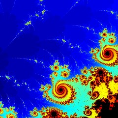
OK,that was a Julia set (different starting points, same formula). What about a counterpart to the Mandelbrot set? I looked at where c is the control parameter. I start with and iterate:
Zooming in shows the same kind of motif copies of Julia sets as we see in the quadratic Mandelbrot set:
In fact, zooming in as above in the counterpart to the “seahorse valley” shows a remarkable similarity.
During a recent party I got asked the question “Since has an infinite decimal expansion, does that mean the collected works of Shakespeare (suitably encoded) are in it somewhere?”
My first response was to point out that infinite decimal expressions are not enough: obviously is a Shakespeare-free number (unless we have a bizarre encoding of the works in the form of all threes). What really matters is whether the number is suitably random. In mathematics this is known as the question about whether pi is a normal number.
This led to a second issue: what is the distribution of the Shakespeare-containing numbers?
We can encode Shakespeare in many ways. As an ASCII text the works take up 5.3 MB. One can treat this as a sequence of 7-bit characters and the works as 37,100,000 bits, or 11,168,212 decimal digits. A simple code where each pair of digits encode a character would encode 10,600,000 digits. This allows just a 100 character alphabet rather than a 127 character alphabet, but is likely OK for Shakespeare: we can use the ASCII code minus 32, for example.
If we denote the encoded works of Shakespeare by , all numbers of the form are Shakespeare-containing.
They form a rather tiny interval: since the works start with ‘The’, starts as “527269…” and the interval lies inside the interval , a mere millionth of . The actual interval is even shorter.
But outside that interval there are numbers of the form , where is a digit different from the starting digit of and anything else. So there are 9 such second level intervals, each ten times thinner than the first level interval.
This pattern continues, with the intervals at each level ten times thinner but also 9 times as numerous. This is fairly similar to the Cantor set and gives rise to a fractal. But since the intervals are very tiny it is hard to see.
One way of visualizing this is to assume the weird encoding , so all numbers containing the digit 3 in the decimal expansion are Shakespearian and the rest are Shakespeare-free.
Distribution of Shakespeare-free numbers in the unit interval, assuming Shakespeare’s collected works are encoded as the digit “3”.
The fractal dimension of this Shakespeare-free set is . This is less than 1: most points are Shakespearian and in one of the intervals, but since they are thin compared to the line the Shakespeare-free set is nearly one dimensional. Like the Cantor set, each Shakespeare-free number is isolated from any other Shakespeare-free number: there is always some Shakespearian numbers between them.
In the case of the full 5.3MB [Shakespeare] the interval length is around . The fractal dimension of the Shakespeare-free set is , for some tiny . It is very nearly an unbroken line… except for that nearly every point actually does contain Shakespeare.
We have been looking at the unit interval. We can of course look at the entire real line too, but the pattern is similar: just magnify the unit interval pattern by 10, 100, 1000, … times. Somewhere around $10^{10,600,000}$ there are the numbers that have an integer part equal to . And above them are the intervals that start with his works followed by something else, a decimal point and then any decimals. And beyond them there are the numbers…
Shakespeare is common
One way of seeing that Shakespearian numbers are the generic case is to imagine choosing a number randomly. It has probability of being in the level 1 interval of Shakespearian numbers. If not, then it will be in one of the 9 intervals 1/10 long that don’t start with the correct first digit, where the probability of starting with Shakespeare in the second digit is . If that was all there was, the total probability would be . But the 1/10 interval around the first Shakespearian interval also counts: a number that has the right first digit but wrong second digit can still be Shakespearian. So it will add probability.
Another way of thinking about it is just to look at the initial digits: the probability of starting with is , the probability of starting with in position 2 is (the first factor is the probability of not having Shakespeare first), and so on. So the total probability of finding Shakespeare is . So nearly all numbers are Shakespearian.
This might seem strange, since any number you are likely to mention is very likely Shakespeare-free. But this is just like the case of transcendental, normal or uncomputable numbers: they are actually the generic case in the reals, but most everyday numbers belong to the algebraic, non-normal and computable numbers.
It is also worth remembering that while all normal numbers are (almost surely) Shakespearian, there are non-normal Shakespearian numbers. For example, the fractional number is non-normal but Shakespearian. So is We can throw in arbitrary finite sequences of digits between the Shakespeares, biasing numbers as close or far as we want from normality. There is a number that has the digits of plus Shakespeare. And there is a number that looks like until Graham’s number digits, then has a single Shakespeare and then continues. Shakespeare can hide anywhere.
In things of great receipt with case we prove,
Among a number one is reckoned none.
Then in the number let me pass untold,
Though in thy store’s account I one must be -Sonnet 136
Most of the time we encounter probability distributions over the reals, the positive reals, or integers. But one can use the rational numbers as a probability space too.
If you take positive independent integers from some distribution and generate ratios , then those ratios will have a distribution that is a convolution over the rational numbers:
One can of course do the same for non-independent and different distributions of the integers. Oh, and by the way: this whole thing has little to do with ratio distributions (alias slash distributions), which is what happens in the real case.
The authors found closed form solutions for integers distributed as a power-law with an exponential cut-off and for the uniform distribution; unfortunately the really interesting case, the Poisson distribution, doesn’t seem to have a neat closed form solution.
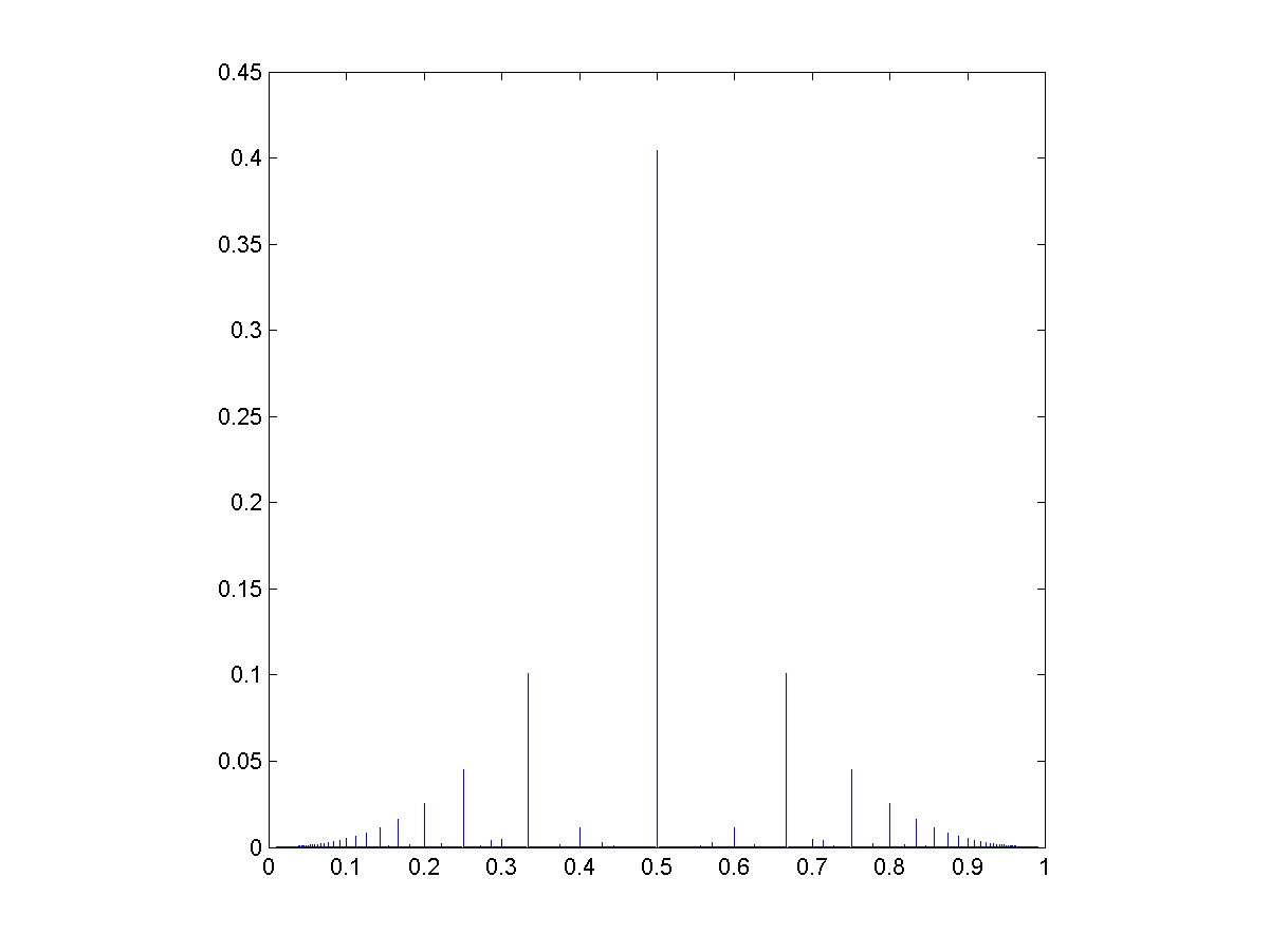
In the case of a uniform distributions on the set they get .
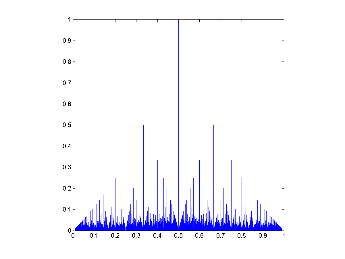
The rational distribution g(a/(a+b))=1/max(a,b) of Trifonov et al.
They note that this is similar to Thomae’s function, a somewhat well-known (and multiply named) counterexample in real analysis. That function is defined as f(p/q)=1/q (where the fraction is in lowest terms). In fact, both graphs have the same fractal dimension of 1.5.
It is easy to generate other rational distributions this way. Using a power law as an input produces a sparser pattern, since the integers going into the ratio tend to be small numbers, putting more probability at simple ratios:
The rational distribution g(a/(a+b))=C(ab)^-2 (rational convolution of two index -2 power-law distributed integers).
If we use exponential distributions the pattern is fairly similar, but we can of course change the exponent to get something that ranges over a lot of numbers, putting more probability at nonsimple ratios where :
The rational distribution of two convolved Exp[0.1] distributions.Not everything has to be neat and symmetric. Taking the ratio of two unequal Poisson distributions can produce a rather appealing pattern:
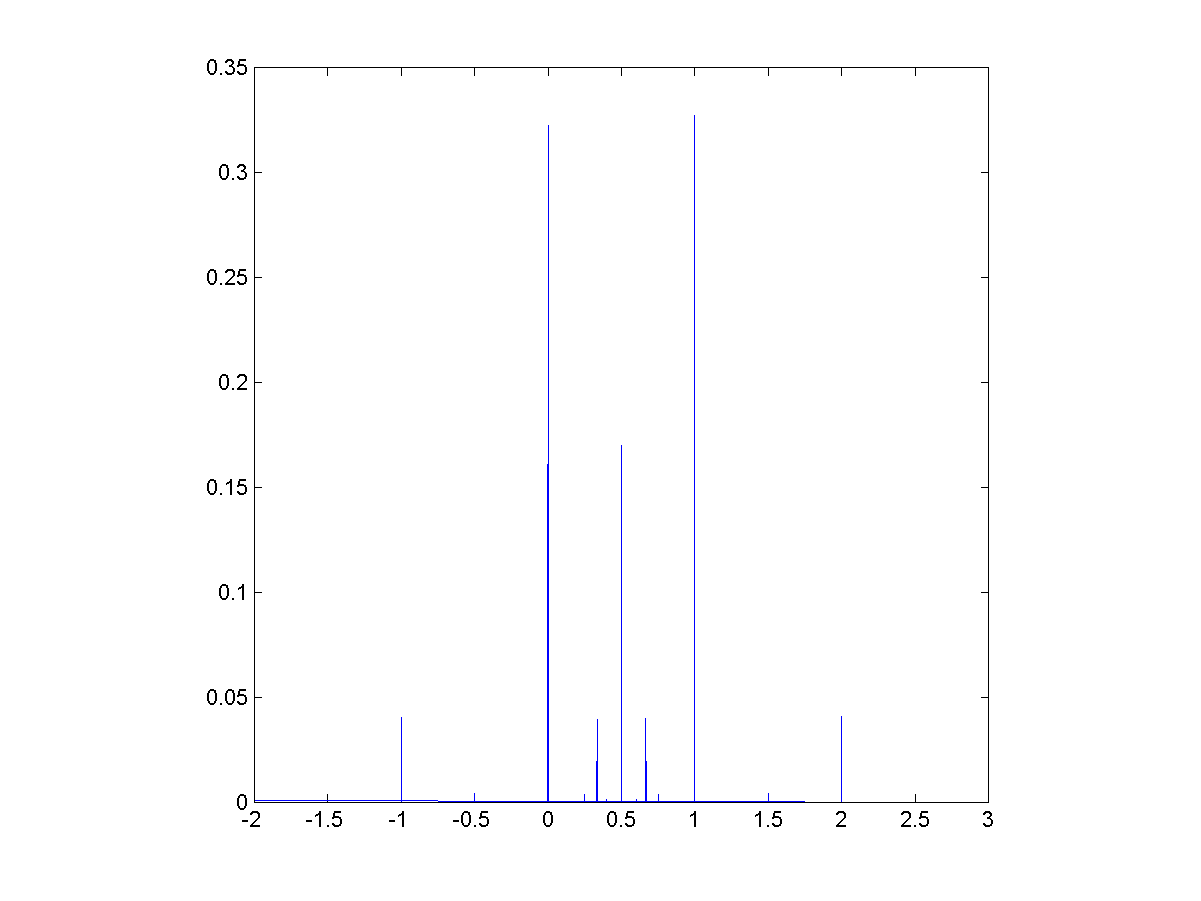
Rational distribution of ratio between a Poisson[10] and a Poisson[5] variable.Of course, full generality would include ratios of non-positive numbers. Taking ratios of normal variates rounded to the nearest integer produces a fairly sparse distribution since high numerators or denominators are rare.
Rational distribution of a/(a+b) ratios of normal variates rounded to nearest integer.
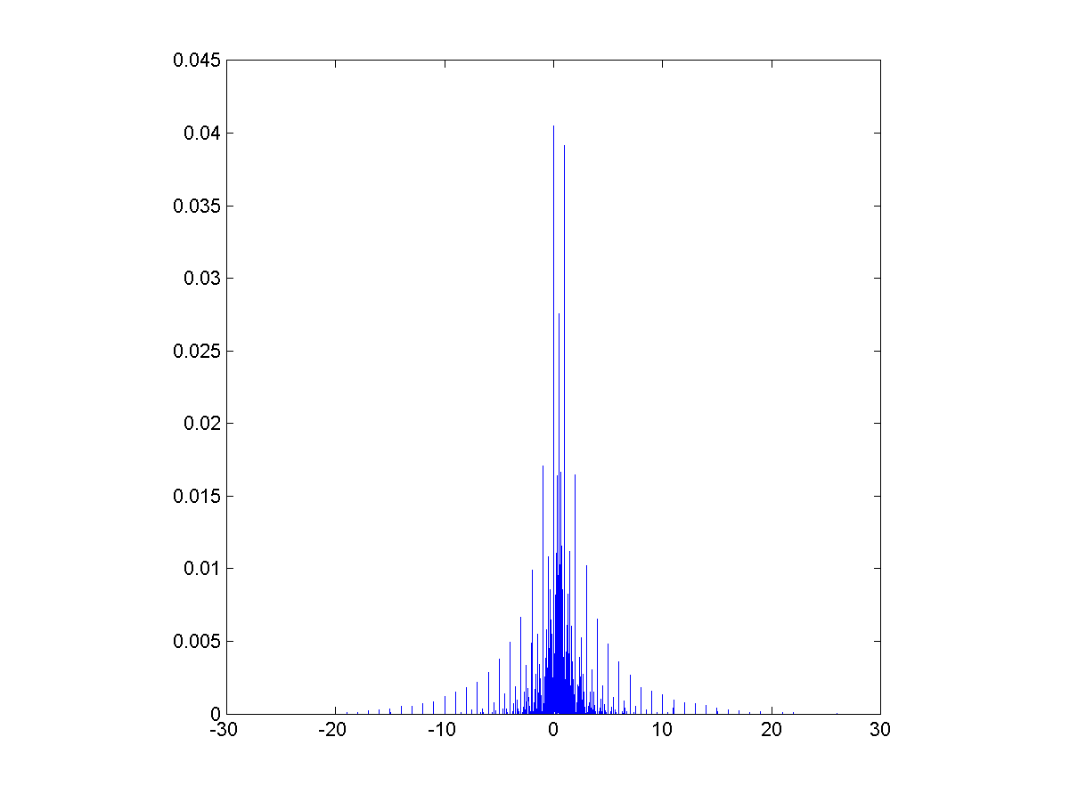
But multiplying the variates by 10 produces a nice distribution.
Rational distribution of a/(a+b) ratios of normal variates that have been multiplied by 10 and rounded.
This approaches the Chauchy distribution as the discretisation gets finer. But note the fun microstructure (very visible in the Poisson case above too), where each peak at a simple ratio is surrounded by a “moat” of low probability. This is reminiscent of the behaviour of roots of random polynomials with integer coefficients (see also John Baez page on the topic).
The rational numbers do tend to induce a fractal recursive structure on things, since most measures on them will tend to put more mass at simple ratios than at complex ratios, but when plotting the value of the ratio everything gets neatly folded together. The lower approximability of numbers near the simple ratios produce moats. Which also suggests a question to ponder further: what role does the über-unapproximable golden ratio have in distributions like these?
In any case, there is something simultaneously ugly and exciting when neat patterns in math just ends for no apparent reason.
Another good example is the story of the Doomsday conjecture. Gwern tells the story well, based on Klarreich: a certain kind of object is found in dimension 2, 6, 14, 30 and 62… aha! They are conjectured to occur in all dimensions. A branch of math was built on this conjecture… and then the pattern failed in dimension 254. Oops.
It is a bit like the opposite case of the number of regular convex polytopes in different dimensions: 1, infinity, 5, 6, 3, 3, 3, 3… Here the series start out crazy, and then becomes very regular.
The volume of a unit sphere increases with dimension until , and then decreases. Leaving the non-intuitiveness of why volumes would shrink aside, the real oddness is that the maximum is for a non-integer dimension. We might argue that the formula is needlessly general and only the integer values count, but many derivations naturally bring in the Gamma function and hence the possibility of non-integer values.
Another association is to this integral problem: given a set of integers , is the integral ? As shown in Moore and Mertens, this is NP-complete. Here the strangeness is that integrals normally are pretty well behaved. It seems absurd that a particular not very scary trigonometric integral should require exponential work to analyze. But in fact, multivariate integrals are NP-hard to approximate, and calculating the volume of a n-dimensional polytope is actually #P-complete.
We tend to assume that mathematics is smoother and more regular than reality. Everything is regular and exceptionless because it is generated by universal rules… except when it isn’t. The rules often act as constraints, and when they do not mesh exactly odd things happen. Similarly we may assume that we know what problems are hard or not, but this is an intuition built in our own world rather than the world of mathematics. Finally, some mathematical truths maybe just are. As Gregory Chaitin has argued, some things in math are irreducible; there is no real reason (at least in the sense of a comprehensive explanation) for why they are true.
Mathematical anti-beauty can be very deep. Maybe it is like the insects, rot and other memento mori in classical still life paintings: a deviation from pleasantness and harmony that adds poignancy and a bit of drama. Or perhaps more accurately, it is wabi-sabi.
 at the point with maximal distance
 ") from the border.
from the border.") , which is then updated
, which is then updated  \leftarrow \min(d(x,y), D(x,y))") where
where ") is the distance to the circle. This trades exactness for some discretization error, but it can easily handle nearly arbitrary shapes.
is the distance to the circle. This trades exactness for some discretization error, but it can easily handle nearly arbitrary shapes.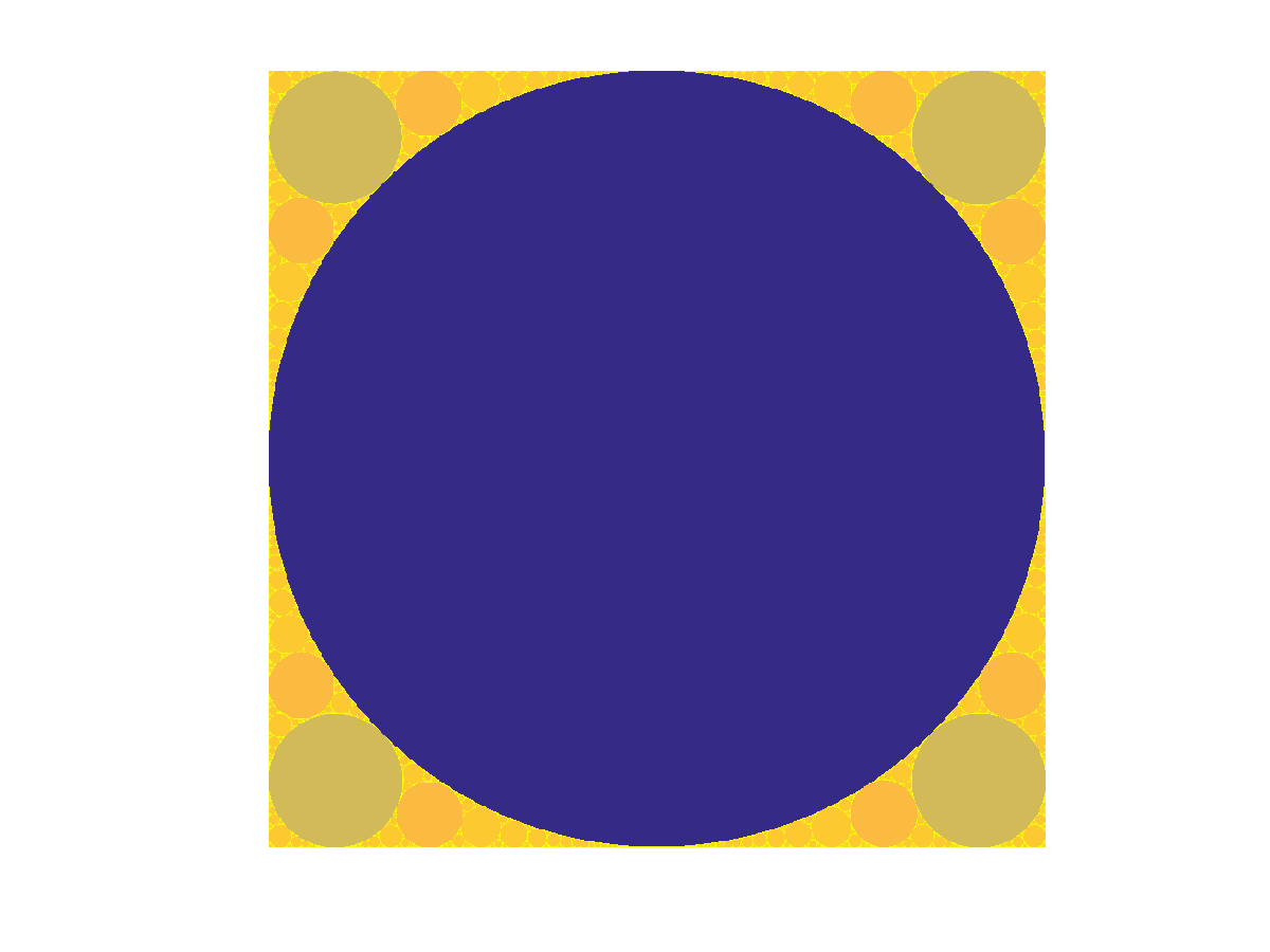
 .
.
\propto r^-\delta") as we approach zero, with
as we approach zero, with  . This is unsurprising: given a generic curved triangle, the inscribed circle will be a fraction of the radii of the bordering circles. If one looks at
  is the Hausdorff dimension of the gasket.
 .
.
 we get sponge-like fractals: these are relatives to the Menger sponge and the Cantor set. The domain gets an infinity of circles punched out of itself, with a total area approaching the area of the domain, so the total measure goes to zero.


 .
.dx\right)dx\right)dx") .
. , the x in the second will be integrated twice
  , and so on.
=\int f(x)+\left(\int f(x)+\left(\int f(x)+\left(\ldots\right)dx\right)dx\right)dx = \sum_{n=1}^\infty \int^n f(x) dx") .
.=f(x)+I(x)") .
.=\sin(kx)") we get the sum
we get the sum =-\cos(kx)/k-\sin(kx)/k^2+\cos(kx)/k^3+\sin(x)/k^4-\cos(kx)/k^5-\ldots") . For
. For  we end up with
 =\sum_{n=0}^\infty 1/k^{4n+2} - \sum_{n=0}^\infty 2/k^{4n+1}") . The differential equation has solution
. The differential equation has solution =ce^x-\sin(kx)/(k^2+1) - k\cos(kx)/(k^2+1)") . Setting
. Setting  the integral is clearly zero, so
  . Tying it together we get:
") .
.=\int x \int x \int x \ldots dx dx dx") . However, we can turn it into a differential equation:
. However, we can turn it into a differential equation: =x I(x)") which has the well known solution
which has the well known solution =ce^{x^2/2}") . Same thing for
. Same thing for =ce^{-\cos(kx)/k}") . Since we are running indefinite integrals we get those pesky constants.
. Since we are running indefinite integrals we get those pesky constants.=1/x") gives
gives =cx") . If we set
. If we set  we get the mildly amusing and in retrospect obvious formula
 .
.=\int\sqrt{\int\sqrt{\int\sqrt{\ldots} dx} dx} dx") , where the differential equation becomes
, where the differential equation becomes  with the solution
 =(1/4)(c^2 + 2cx + x^2)") . A surprisingly simple solution to a weird-looking integral. In a similar vein:
. A surprisingly simple solution to a weird-looking integral. In a similar vein:=\int\sin\left(\int\sin\left(\int\sin\left(\ldots\right)dx\right) dx\right) dx")
=\int \exp\left(\int \exp\left(\int \exp\left(\ldots \right) dx \right) dx \right) dx")
=\int \left(\int \left(\int \left(\ldots \right)^2 dx \right)^2 dx \right)^2 dx")
=\int W\left(\int W\left(\int W\left(\ldots \right) dx \right) dx \right) dx") , then
, then }1/W(t) dt + c") .
. is holomorphic, then
=\Re\left(\int_{z_0}^z f(1-g^2)/2 dz\right)")
=\Re\left(\int_{z_0}^z if(1+g^2)/2 dz\right)")
=\Re\left(\int_{z_0}^z fg dz\right)")
,Y(z),Z(z))") .
.") .
. to different points
  in the complex plane. Let us start with the simple case of
 >1/2") .
.
 – a rather neat residue!) to the coordinates: a translation in the positive y-direction. If we extend the surface by going an extra turn clockwise or counterclockwise a number of times, we get copies that attach seamlessly.
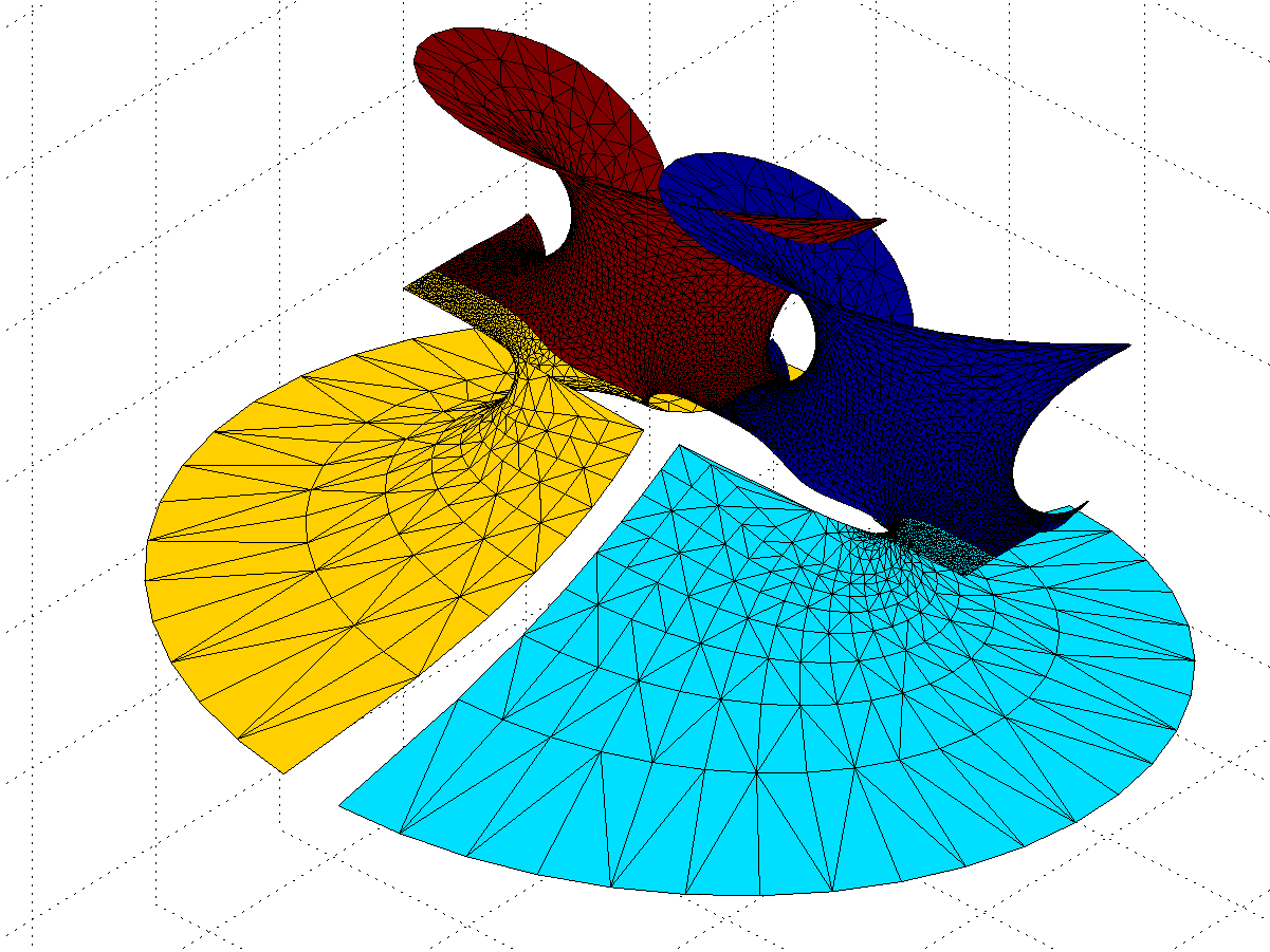
 . They also introduce residues along the y-direction, but different ones from the z=0 – their extensions of the surface will be out of phase with each other, making the fully extended surface fantastically self-intersecting and confusing.
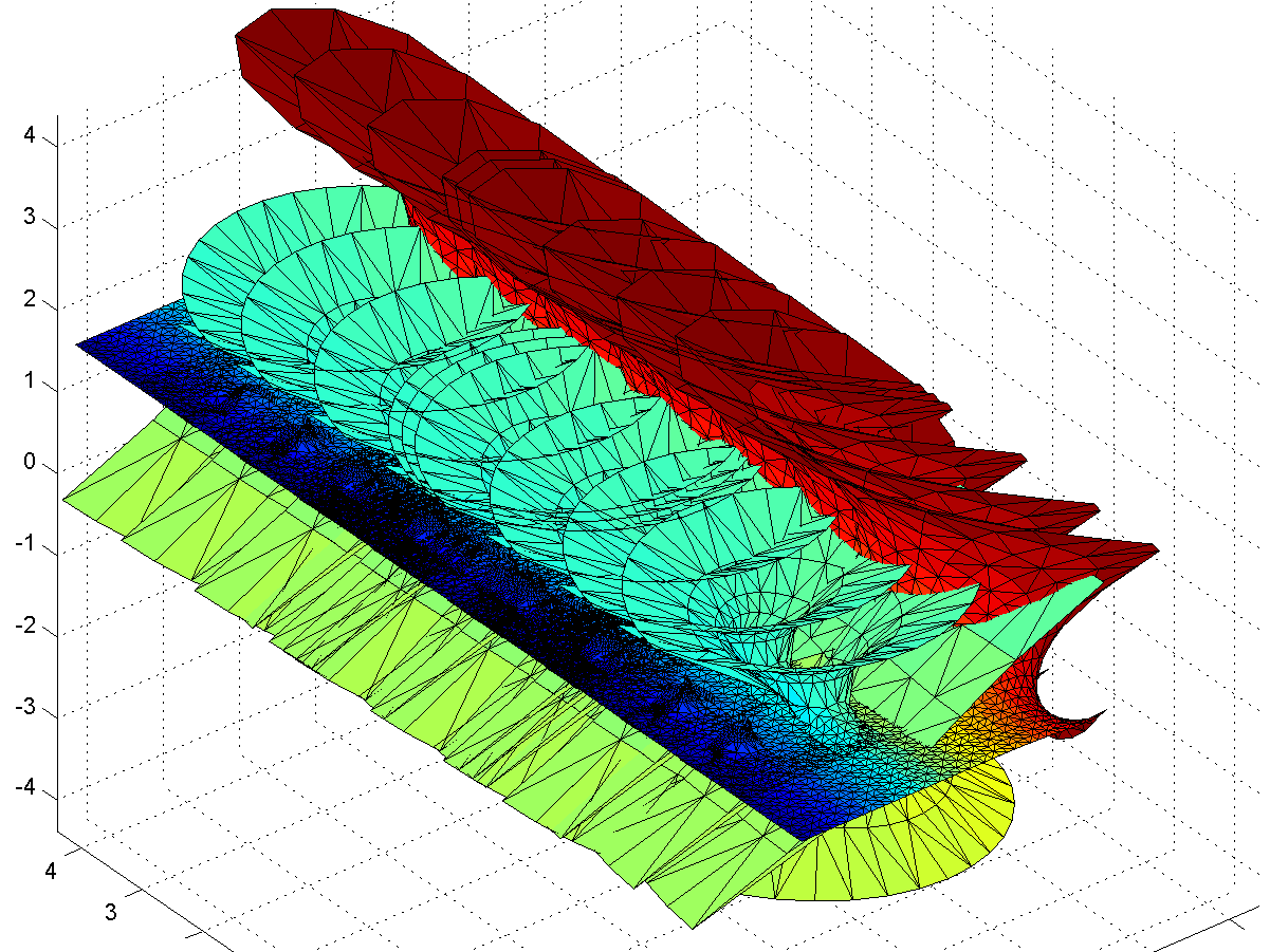
") is nicely behaved and looks very much like the Enneper surface near zero, with “wings” that oscillate ever more wildly as we move towards the negative reals. No doubt there are other beautiful things to look for in the vicinity.
is nicely behaved and looks very much like the Enneper surface near zero, with “wings” that oscillate ever more wildly as we move towards the negative reals. No doubt there are other beautiful things to look for in the vicinity.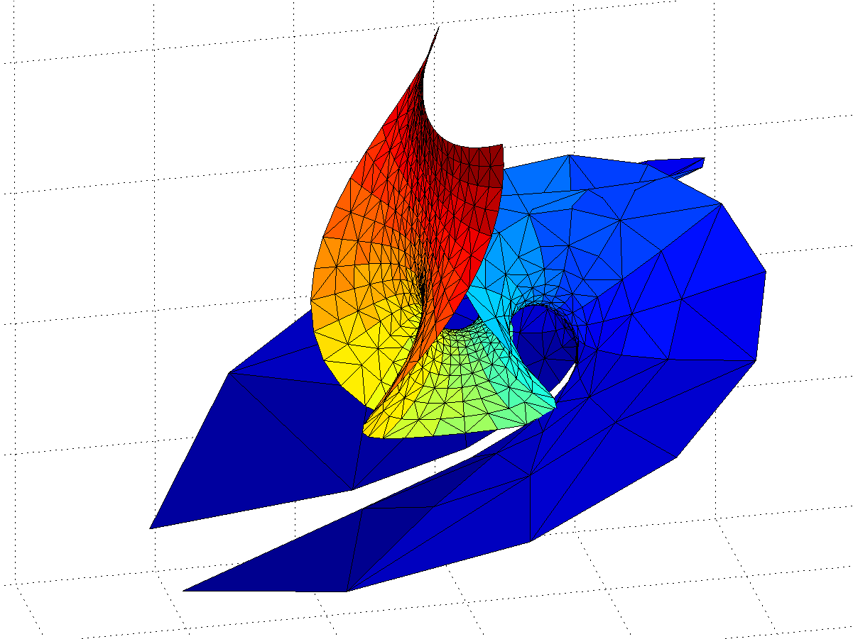
=\int_0^\infty t^{z-1}e^{-t} dt") , the continuous generalization of the factorial. While it grows rapidly for positive reals, it has fun poles for the negative integers and is generally complex.
, the continuous generalization of the factorial. While it grows rapidly for positive reals, it has fun poles for the negative integers and is generally complex. ") . The result is a nice fractal, with some domains approaching 1, and others running off to infinity.
. The result is a nice fractal, with some domains approaching 1, and others running off to infinity.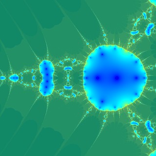
 . Zooming in a bit more reveals neat self-similar patterns with alternating “beans”:
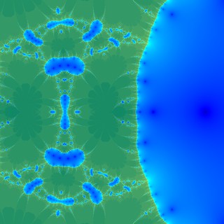
") where c is the control parameter. I start with
where c is the control parameter. I start with 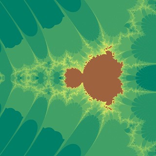
 has an infinite decimal expansion, does that mean the collected works of Shakespeare (suitably encoded) are in it somewhere?”
 is a Shakespeare-free number (unless we have a bizarre encoding of the works in the form of all threes). What really matters is whether the number is suitably random. In mathematics this is known as the question about whether pi is a
 ![[Shakespeare]](http://s0.wp.com/latex.php?latex=%5BShakespeare%5D&bg=ffffff&fg=000000&s=0 "[Shakespeare]") , all numbers of the form
, all numbers of the form ![0.[Shakespeare]xxxxx\ldots](http://s0.wp.com/latex.php?latex=0.%5BShakespeare%5Dxxxxx%5Cldots+&bg=ffffff&fg=000000&s=0 "0.[Shakespeare]xxxxx\ldots") are Shakespeare-containing.
are Shakespeare-containing.![[0. 527269000\ldots , 0.52727]](http://s0.wp.com/latex.php?latex=%5B0.+527269000%5Cldots+%2C+0.52727%5D&bg=ffffff&fg=000000&s=0 "[0. 527269000\ldots , 0.52727]") , a mere millionth of
, a mere millionth of ![[0,1]](http://s0.wp.com/latex.php?latex=%5B0%2C1%5D&bg=ffffff&fg=000000&s=0 "[0,1]") . The actual interval is even shorter.
. The actual interval is even shorter.![0.y[Shakespeare]xxxx\ldots](http://s0.wp.com/latex.php?latex=0.y%5BShakespeare%5Dxxxx%5Cldots+&bg=ffffff&fg=000000&s=0 "0.y[Shakespeare]xxxx\ldots") , where
, where  is a digit different from the starting digit of
  anything else. So there are 9 such second level intervals, each ten times thinner than the first level interval.
![[Shakespeare]=3](http://s0.wp.com/latex.php?latex=%5BShakespeare%5D%3D3&bg=ffffff&fg=000000&s=0 "[Shakespeare]=3") , so all numbers containing the digit 3 in the decimal expansion are Shakespearian and the rest are Shakespeare-free.
, so all numbers containing the digit 3 in the decimal expansion are Shakespearian and the rest are Shakespeare-free.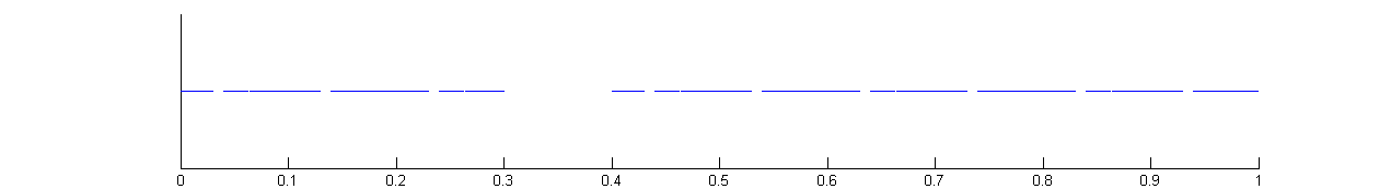
/\log(10)\approx 0.9542") . This is less than 1: most points are Shakespearian and in one of the intervals, but since they are thin compared to the line the Shakespeare-free set is nearly one dimensional. Like the Cantor set, each Shakespeare-free number is isolated from any other Shakespeare-free number: there is always some Shakespearian numbers between them.
. This is less than 1: most points are Shakespearian and in one of the intervals, but since they are thin compared to the line the Shakespeare-free set is nearly one dimensional. Like the Cantor set, each Shakespeare-free number is isolated from any other Shakespeare-free number: there is always some Shakespearian numbers between them. . The fractal dimension of the Shakespeare-free set is
 /\log(10^{10,600,600}) \approx 1-\epsilon") , for some tiny
, for some tiny  . It is very nearly an unbroken line… except for that nearly every point actually does contain Shakespeare.
![[Shakespeare][Shakespeare]xxx\ldots](http://s0.wp.com/latex.php?latex=%5BShakespeare%5D%5BShakespeare%5Dxxx%5Cldots&bg=ffffff&fg=000000&s=0 "[Shakespeare][Shakespeare]xxx\ldots") numbers…
numbers… of being in the level 1 interval of Shakespearian numbers. If not, then it will be in one of the 9 intervals 1/10 long that don’t start with the correct first digit, where the probability of starting with Shakespeare in the second digit is
 S+(9/10^2)S+\ldots = 10S<1") . But the 1/10 interval around the first Shakespearian interval also counts: a number that has the right first digit but wrong second digit can still be Shakespearian. So it will add probability.
. But the 1/10 interval around the first Shakespearian interval also counts: a number that has the right first digit but wrong second digit can still be Shakespearian. So it will add probability.S") (the first factor is the probability of not having Shakespeare first), and so on. So the total probability of finding Shakespeare is
(the first factor is the probability of not having Shakespeare first), and so on. So the total probability of finding Shakespeare is S + (1-S)^2S + (1-S)^3S + \ldots = S/(1-(1-S))=1") . So nearly all numbers are Shakespearian.
. So nearly all numbers are Shakespearian.![0.[Shakespeare]000\ldots](http://s0.wp.com/latex.php?latex=0.%5BShakespeare%5D000%5Cldots+&bg=ffffff&fg=000000&s=0 "0.[Shakespeare]000\ldots") is non-normal but Shakespearian. So is
is non-normal but Shakespearian. So is ![0.[Shakespeare][Shakespeare][Shakespeare]\ldots](http://s0.wp.com/latex.php?latex=0.%5BShakespeare%5D%5BShakespeare%5D%5BShakespeare%5D%5Cldots+&bg=ffffff&fg=000000&s=0 "0.[Shakespeare][Shakespeare][Shakespeare]\ldots") We can throw in arbitrary finite sequences of digits between the Shakespeares, biasing numbers as close or far as we want from normality. There is a number
We can throw in arbitrary finite sequences of digits between the Shakespeares, biasing numbers as close or far as we want from normality. There is a number ![0.[Shakespeare]3141592\ldots](http://s0.wp.com/latex.php?latex=0.%5BShakespeare%5D3141592%5Cldots&bg=ffffff&fg=000000&s=0 "0.[Shakespeare]3141592\ldots") that has the digits of
that has the digits of 
") and generate ratios
and generate ratios ") , then those ratios will have a distribution that is a convolution over the rational numbers:
, then those ratios will have a distribution that is a convolution over the rational numbers:  = g(a/(a+b)) = \sum_{m=0}^\infty \sum_{n=0}^\infty f(m) g(n) \delta \left(\frac{a}{a+b} - \frac{m}{m+n} \right ) = \sum_{t=0}^\infty f(ta)f(tb)")
 they get
 ) = (1/L^2) \lfloor L/\max(a,b) \rfloor") .
.
 where
where  :
:![The rational distribution of two convolved Exp[0.1] distributions.](http://aleph.se/andart2/wp-content/uploads/2014/09/trifonovexp01.png)
![Rational distribution of ratio between a Poisson[10] and a Poisson[5] variable.](http://aleph.se/andart2/wp-content/uploads/2014/09/trifonovpoiss105.png)
=sin(x)/x") for
for  and defined to be 1 for
  dx = \pi/2") ,
, sinc(x/3) dx = \pi/2") ,
, sinc(x/3) sinc(x/5) dx = \pi/2") .
. sinc(x/3) sinc(x/5) \cdots sinc(x/13) dx = \pi/2") .
. sinc(x/3) sinc(x/5)")
 sinc(x/15) dx")

 – nearly a half, but not quite.
 dimensions. A branch of math was built on this conjecture… and then the pattern failed in dimension 254. Oops.
 =\frac{\pi^{n/2}r^n}{\Gamma(1+n/2)}")
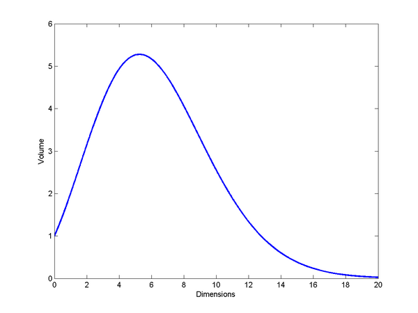
 , and then decreases. Leaving the non-intuitiveness of why volumes would shrink aside, the real oddness is that the maximum is for a non-integer dimension. We might argue that the formula is needlessly general and only the integer values count, but many derivations naturally bring in the Gamma function and hence the possibility of non-integer values.
 , is the integral
  d\theta = 0") ? As shown in
? As shown in