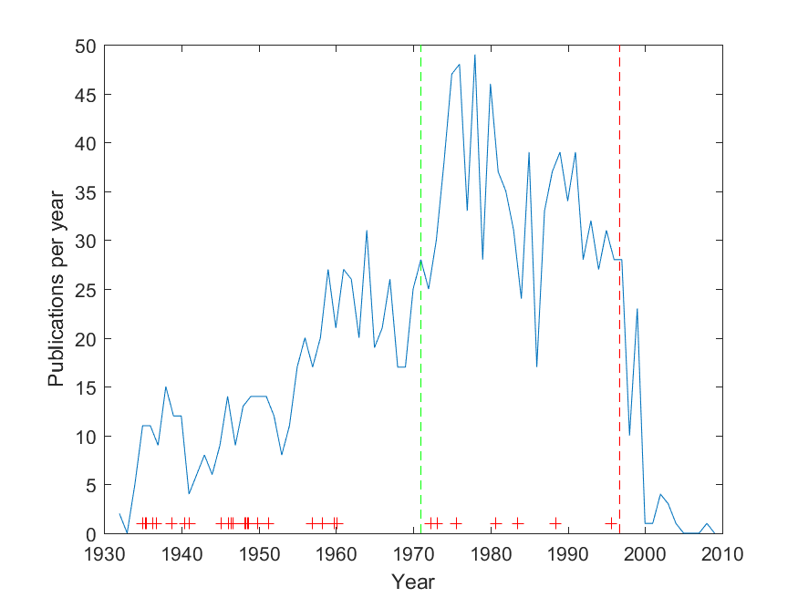
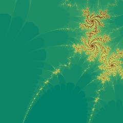
During my work on the Paris talk I began to wonder whether Paul Erdős (who I used as an example of a respected academic who used cognitive enhancers) could actually have been shown to have benefited from his amphetamine use, which began in 1971 according to Hill (2004). One way of investigating is his publication record: how many papers did he produce per year before or after 1971? Here is a plot, based on Jerrold Grossman’s 2010 bibliography:
Productivity of Paul Erdos over his life. Green dashed line: amphetamine use, red dashed line: death. Crosses mark named concepts.
The green dashed line is the start of amphetamine use, and the red dashed life is the date of death. Yes, there is a fairly significant posthumous tail: old mathematicians never die, they just asymptote towards zero. Overall, the later part is more productive per year than the early part (before 1971 the mean and standard deviation was 14.6±7.5, after 24.4±16.1; a Kruskal-Wallis test rejects that they are the same distribution, p=2.2e-10).
This does not prove anything. After all, his academic network was growing and he moved from topic to topic, so we cannot prove any causal effect of the amphetamine: for all we know, it might have been holding him back.
One possible argument might be that he did not do his best work on amphetamine. To check this, I took the Wikipedia article that lists things named after Erdős, and tried to find years for the discovery/conjecture. These are marked with red crosses in the diagram, slightly jittered. We can see a few clusters that may correspond to creative periods: one in 35-41, one in 46-51, one in 56-60. After 1970 the distribution was more even and sparse. 76% of the most famous results were done before 1971; given that this is 60% of the entire career it does not look that unlikely to be due to chance (a binomial test gives p=0.06).
Again this does not prove anything. Maybe mathematics really is a young man’s game, and we should expect key results early. There may also have been more time to recognize and name results from the earlier career.
In the end, this is merely a statistical anecdote. It does show that one can be a productive, well-renowned (if eccentric) academic while on enhancers for a long time. But given the N=1, firm conclusions or advice are hard to draw.
Erdős’s friends worried about his drug use, and in 1979 Graham bet Erdős $500 that he couldn’t stop taking amphetamines for a month. Erdős accepted, and went cold turkey for a complete month. Erdős’s comment at the end of the month was “You’ve showed me I’m not an addict. But I didn’t get any work done. I’d get up in the morning and stare at a blank piece of paper. I’d have no ideas, just like an ordinary person. You’ve set mathematics back a month.” He then immediately started taking amphetamines again. (Hill 2004)
One of the first fractals I ever saw was the Apollonian gasket, the shape that emerges if you draw the circle internally tangent to three other tangent circles. It is somewhat similar to the Sierpinski triangle, but has a more organic flair. I can still remember opening my copy of Mandelbrot’s The Fractal Geometry of Nature and encountering this amazing shape. There is a lot of interesting things going on here.
Here is a simple algorithm for generating related circle packings, trading recursion for flexibility:
Start with a domain and calculate the distance to the border for all interior points.
Place a circle of radius at the point with maximal distance from the border.
Recalculate the distances, treating the new circle as a part of the border.
Repeat (2-3) until the radius becomes smaller than some tolerance.
This is easily implemented in Matlab if we discretize the domain and use an array of distances , which is then updated where is the distance to the circle. This trades exactness for some discretization error, but it can easily handle nearly arbitrary shapes.
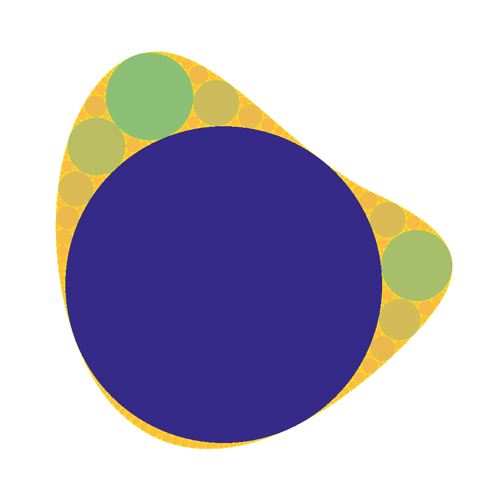
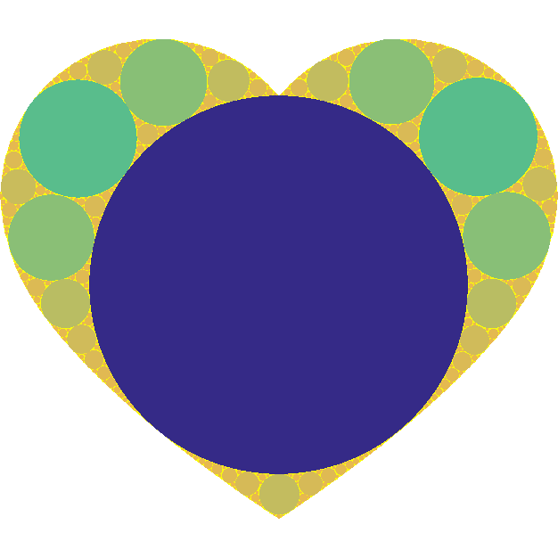
Apollonian circle packing in square.Apollonian circle packing in blob.Apollonian circle packing in heart.
It is interesting to note that the topology is Apollonian nearly everywhere: as soon as three circles form a curvilinear triangle the interior will be a standard gasket if .
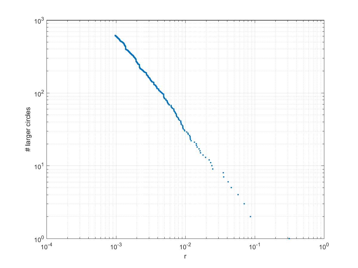
Number of circles larger than a certain radius in packing in blob shape.
In the above pictures the first circle tends to dominate. In fact, the size distribution of circles is a power law: the number of circles larger than r grows as as we approach zero, with . This is unsurprising: given a generic curved triangle, the inscribed circle will be a fraction of the radii of the bordering circles. If one looks at integral circle packings it is possible to see that the curvatures of subsequent circles grow quadratically along each “horn”, but different “horns” have different growths. Because of the curvature the self-similarity is nontrivial: there is actually, as far as I know, still no analytic expression of the fractal dimension of the gasket. Still, one can show that the packing exponent is the Hausdorff dimension of the gasket.
Anyway, to make the first circle less dominant we can either place a non-optimal circle somewhere, or use lower .
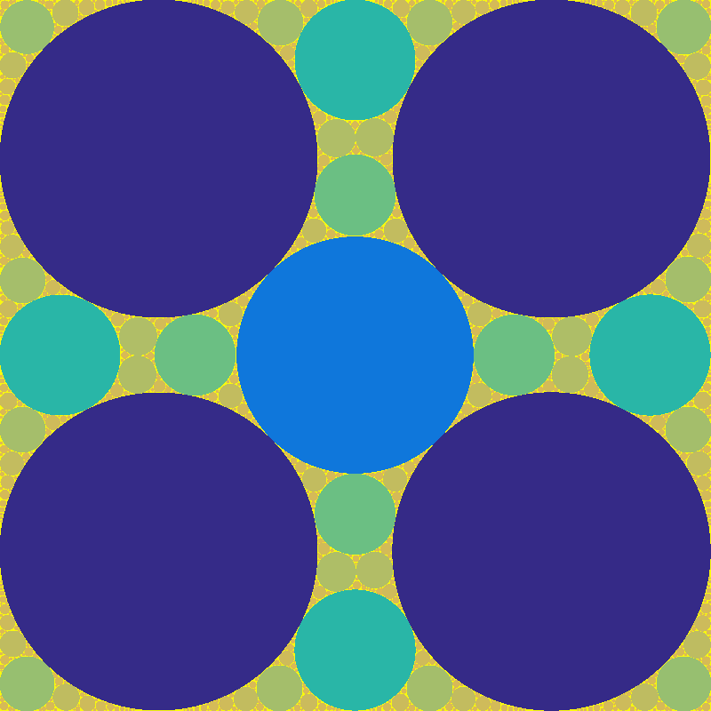
Apollonian packing in square with central circle of radius 1/6.
If we place a circle in the centre of a square with a radius smaller than the distance to the edge, it gets surrounded by larger circles.
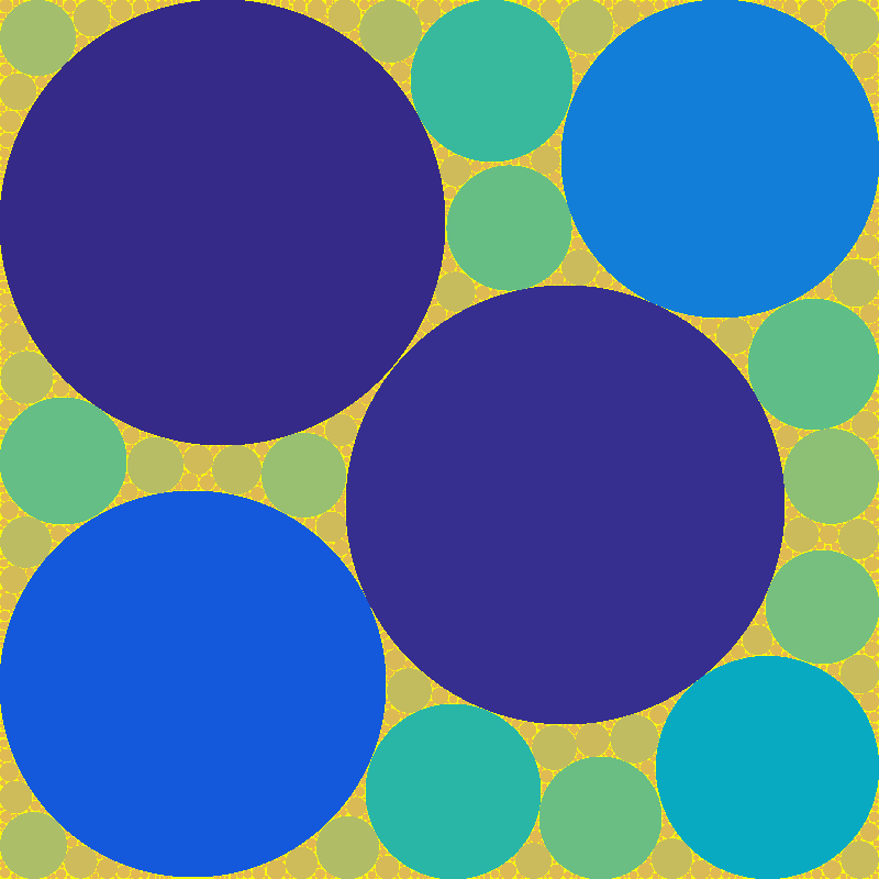
Randomly started Apollonian packing.
If the circle is misaligned, it is no problem for the tiling: any discrepancy can be filled with sufficiently small circles. There is however room for arbitrariness: when a bow-tie-shaped region shows up there are often two possible ways of placing a maximal circle in it, and whichever gets selected breaks the symmetry, typically producing more arbitrary bow-ties. For “neat” arrangements with the right relationships between circle curvatures and positions this does not happen (they have circle chains corresponding to various integer curvature relationships), but the generic case is a mess. If we move the seed circle around, the rest of the arrangement both show random jitter and occasional large-scale reorganizations.
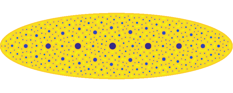
When we let we get sponge-like fractals: these are relatives to the Menger sponge and the Cantor set. The domain gets an infinity of circles punched out of itself, with a total area approaching the area of the domain, so the total measure goes to zero.
Apollonian packing with alpha=0.5.
That these images have an organic look is not surprising. Vascular systems likely grow by finding the locations furthest away from existing vascularization, then filling in the gaps recursively (OK, things are a bit more complex).
Apollonian packing with alpha=1/4.Apollonian packing with alpha=0.1.
Recently I encountered a specialist Wiki. I pressed “random page” a few times, and got a repeat page after 5 tries. How many pages should I expect this small wiki to have?
We can compare this to the German tank problem. Note that it is different; in the tank problem we have a maximum sample (maybe like the web pages on the site were numbered), while here we have number of samples before repetition.
We can of course use Bayes theorem for this. If I get a repeat after random samples, the posterior distribution of , the number of pages, is .
If I randomly sample from pages, the probability of getting a repeat on my second try is , on my third try , and so on: . Of course, there has to be more pages than , otherwise a repeat must have happened before step , so this is valid for . Otherwise, for .
The prior needs to be decided. One approach is to assume that websites have a power-law distributed number of pages. The majority are tiny, and then there are huge ones like Wikipedia; the exponent is close to 1. This gives us . Note the appearance of the Riemann zeta function as a normalisation factor.
We can calculate by summing over the different possible : .
Putting it all together we get for . The posterior distribution of number of pages is another power-law. Note that the dependency on is rather subtle: it is in the support of the distribution, and the upper limit of the partial sum.
What about the expected number of pages in the wiki? . The expectation is the ratio of the zeta functions of and , minus the first terms of their series.
Distribution of P(N|5) for [latex]\alpha=1.1[/latex].
So, what does this tell us about the wiki I started with? Assuming (close to the behavior of big websites), it predicts . If one assumes a higher the number of pages would be 7 (which was close to the size of the wiki when I looked at it last night – it has grown enough today for k to equal 13 when I tried it today).
Expected number of pages given k random views before a repeat.
So, can we derive a useful rule of thumb for the expected number of pages? Dividing by shows that approaches proportionality, especially for larger :
E(N|k)/k as a function of k.
So a good rule of thumb is that if you get pages before a repeat, expect between and pages on the site. However, remember that we are dealing with power-laws, so the variance can be surprisingly high.
The classification of tie knots is not in itself important, but having a nice notation helps for specifying how to tie them. And the links to languages and finite state machines are cool. The big research challenge is understanding how knot façades are to be modelled and judged.
What about nested/continued integrals? Here is a simple one:
.
The way to see this is to recognize that the x in the first integral is going to integrate to , the x in the second will be integrated twice , and so on.
In general additive integrals of this kind turn into sums (assuming convergence, handwave, handwave…):
.
On the other hand, .
So if we insert we get the sum . For we end up with . The differential equation has solution . Setting the integral is clearly zero, so . Tying it together we get:
.
Things are trickier when the integrals are multiplicative, like . However, we can turn it into a differential equation: which has the well known solution . Same thing for , giving us . Since we are running indefinite integrals we get those pesky constants.
Plugging in gives . If we set we get the mildly amusing and in retrospect obvious formula
.
We can of course mess things up further, like , where the differential equation becomes with the solution . A surprisingly simple solution to a weird-looking integral. In a similar vein:
(that is, you get an implicit but well defined expression for the (x,I(x)) values. With Lambert, the x and y axes always tend to switch place).
[And yes, convergence is handwavy in this essay. I think the best way of approaching it is to view the values of these integrals as the functions invariant under the functional consisting of the integral and its repeated function: whether nearby functions are attracted to it (or not) under repeated application of the functional depends on the case. ]
The gamma function has a long and interesting history (check out (Davis 1963) excellent review), but one application does not seem to have shown up: minimal surfaces.
A minimal surface is one where the average curvature is always zero; it bends equally in two opposite directions. This is equivalent to having the (locally) minimal area given its boundary: such surfaces are commonly seen as soap films stretched from frames. There exists a rich theory for them, linking them to complex analysis through the Enneper-Weierstrass representation: if you have a meromorphic function g and an analytic function f such that is holomorphic, then
produces a minimal surface .
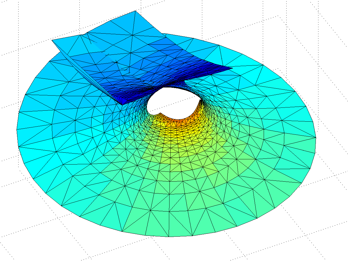
When plugging in the hyperbolic tangent as g and using f=1 I got a new and rather nifty surface a few years back. What about plugging in the gamma function? Let .
We integrate from the regular point to different points in the complex plane. Let us start with the simple case of .
Gamma function minimal surface for z in 0.5<Re(z)<3.5, -8<Im(z)
The surface is a billowing strip, and as we include z with larger and larger real parts the amplitude of the oscillations grow rapidly, making it self-intersect. The behaviour is somewhat similar to the Catalan minimal surface, except that we only get one period. If we go to larger imaginary parts the surface approaches a horizontal plane. OK, the surface is a plane with some wild waves, right?
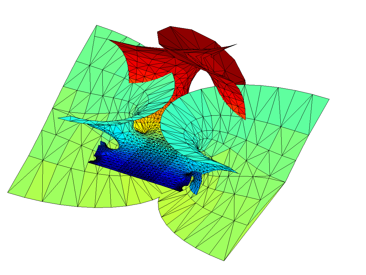
Not so fast, we have not looked at the mess for Re(z)<0. First, let’s examine the area around the z=0 singularity. Since the values of the integrand blows up close to it, they produce a surface expanding towards infinity – very similar to a catenoid. Indeed, catenoid ends tend to show up where there are poles. But this one doesn’t close exactly: for re(z)<0 there is some overshoot producing a self-intersecting plane-like strip.
Gamma function minimal surface close to the z=0 singularity. Colour denotes Re(z). Integration contours from 1 to z run clockwise for Im(z)<0 and counterclockwise for Im(z)>0.
The problem is of course the singularity: when integrating in the complex plane we need to avoid them, and depending on the direction we go around them we can get a complex phase that gives us an entirely different value of the function. In this case the branch cut corresponds to the real line: integrating clockwise or counter-clockwise around z=0 to the same z gives different values. In fact, a clockwise turn adds [3.6268i, 3.6268, 6.2832i] (which looks like – a rather neat residue!) to the coordinates: a translation in the positive y-direction. If we extend the surface by going an extra turn clockwise or counterclockwise a number of times, we get copies that attach seamlessly.
Gamma minimal surface extended by integration paths between the -1 and 0 singularities (blue patches).
Gamma minimal surface patch that can be repeated by translation along the y-axis. Colour denotes Re(z).
OK, we have a surface with some planar strips that turn wobbly and self-intersecting in the x-direction, with elliptic catenoid ends repeating along the y-direction due to the z=0 singularity. Going down the negative x-direction things look plane between the catenoids… except of course for the catenoids due to all the other singularities for . They also introduce residues along the y-direction, but different ones from the z=0 – their extensions of the surface will be out of phase with each other, making the fully extended surface fantastically self-intersecting and confusing.
Gamma function minimal surface extended by integrating around poles.
So, I think we have a simple answer to why the gamma function minimal surface is not well known: it is simply too messy and self-intersecting.
Of course, there may be related nifty surfaces. is nicely behaved and looks very much like the Enneper surface near zero, with “wings” that oscillate ever more wildly as we move towards the negative reals. No doubt there are other beautiful things to look for in the vicinity.
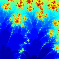
Another of my favourite functions if the Gamma function, , the continuous generalization of the factorial. While it grows rapidly for positive reals, it has fun poles for the negative integers and is generally complex. What happens when you iterate it?
First I started by just applying it to different starting points, . The result is a nice fractal, with some domains approaching 1, and others running off to infinity.
Here I color points that go to infinity in green shades on the number of iterations before they become very large, and the points approaching 1 by . Zooming in a bit more reveals neat self-similar patterns with alternating “beans”:
In the outside regions we have thin tendrils stretching towards infinity. These are familiar to anybody who has been iterating exponentials or trigonometric functions: the combination of oscillation and (super)exponential growth leads to the pattern.
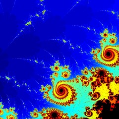
OK,that was a Julia set (different starting points, same formula). What about a counterpart to the Mandelbrot set? I looked at where c is the control parameter. I start with and iterate:
Zooming in shows the same kind of motif copies of Julia sets as we see in the quadratic Mandelbrot set:
In fact, zooming in as above in the counterpart to the “seahorse valley” shows a remarkable similarity.
During a recent party I got asked the question “Since has an infinite decimal expansion, does that mean the collected works of Shakespeare (suitably encoded) are in it somewhere?”
My first response was to point out that infinite decimal expressions are not enough: obviously is a Shakespeare-free number (unless we have a bizarre encoding of the works in the form of all threes). What really matters is whether the number is suitably random. In mathematics this is known as the question about whether pi is a normal number.
This led to a second issue: what is the distribution of the Shakespeare-containing numbers?
We can encode Shakespeare in many ways. As an ASCII text the works take up 5.3 MB. One can treat this as a sequence of 7-bit characters and the works as 37,100,000 bits, or 11,168,212 decimal digits. A simple code where each pair of digits encode a character would encode 10,600,000 digits. This allows just a 100 character alphabet rather than a 127 character alphabet, but is likely OK for Shakespeare: we can use the ASCII code minus 32, for example.
If we denote the encoded works of Shakespeare by , all numbers of the form are Shakespeare-containing.
They form a rather tiny interval: since the works start with ‘The’, starts as “527269…” and the interval lies inside the interval , a mere millionth of . The actual interval is even shorter.
But outside that interval there are numbers of the form , where is a digit different from the starting digit of and anything else. So there are 9 such second level intervals, each ten times thinner than the first level interval.
This pattern continues, with the intervals at each level ten times thinner but also 9 times as numerous. This is fairly similar to the Cantor set and gives rise to a fractal. But since the intervals are very tiny it is hard to see.
One way of visualizing this is to assume the weird encoding , so all numbers containing the digit 3 in the decimal expansion are Shakespearian and the rest are Shakespeare-free.
Distribution of Shakespeare-free numbers in the unit interval, assuming Shakespeare’s collected works are encoded as the digit “3”.
The fractal dimension of this Shakespeare-free set is . This is less than 1: most points are Shakespearian and in one of the intervals, but since they are thin compared to the line the Shakespeare-free set is nearly one dimensional. Like the Cantor set, each Shakespeare-free number is isolated from any other Shakespeare-free number: there is always some Shakespearian numbers between them.
In the case of the full 5.3MB [Shakespeare] the interval length is around . The fractal dimension of the Shakespeare-free set is , for some tiny . It is very nearly an unbroken line… except for that nearly every point actually does contain Shakespeare.
We have been looking at the unit interval. We can of course look at the entire real line too, but the pattern is similar: just magnify the unit interval pattern by 10, 100, 1000, … times. Somewhere around $10^{10,600,000}$ there are the numbers that have an integer part equal to . And above them are the intervals that start with his works followed by something else, a decimal point and then any decimals. And beyond them there are the numbers…
Shakespeare is common
One way of seeing that Shakespearian numbers are the generic case is to imagine choosing a number randomly. It has probability of being in the level 1 interval of Shakespearian numbers. If not, then it will be in one of the 9 intervals 1/10 long that don’t start with the correct first digit, where the probability of starting with Shakespeare in the second digit is . If that was all there was, the total probability would be . But the 1/10 interval around the first Shakespearian interval also counts: a number that has the right first digit but wrong second digit can still be Shakespearian. So it will add probability.
Another way of thinking about it is just to look at the initial digits: the probability of starting with is , the probability of starting with in position 2 is (the first factor is the probability of not having Shakespeare first), and so on. So the total probability of finding Shakespeare is . So nearly all numbers are Shakespearian.
This might seem strange, since any number you are likely to mention is very likely Shakespeare-free. But this is just like the case of transcendental, normal or uncomputable numbers: they are actually the generic case in the reals, but most everyday numbers belong to the algebraic, non-normal and computable numbers.
It is also worth remembering that while all normal numbers are (almost surely) Shakespearian, there are non-normal Shakespearian numbers. For example, the fractional number is non-normal but Shakespearian. So is We can throw in arbitrary finite sequences of digits between the Shakespeares, biasing numbers as close or far as we want from normality. There is a number that has the digits of plus Shakespeare. And there is a number that looks like until Graham’s number digits, then has a single Shakespeare and then continues. Shakespeare can hide anywhere.
In things of great receipt with case we prove,
Among a number one is reckoned none.
Then in the number let me pass untold,
Though in thy store’s account I one must be -Sonnet 136
As iteration formula I choose , where c is a multiplicative constant. Iterating some number like 1 and plotting its fate produces the following “Mandelbrot set” in the c-plane – the colours here do not denote the time until escape to infinity but rather where in the complex plane the point ended up, as a function of c. In a normal Mandelbrot set infinity is an attractive fixed point; here it is just one place in the (extended) complex plane like any other.
“Mandelbrot set” for the hyperbolic tanh function tanh(cz).
The pinkish surroundings of the pattern represent points attracted to the positive solution of . There is of course a corresponding negative solution since tanh is antisymmetric: if z is an attractive fixed point or cycle, so is -z. So the dynamics is always bistable.
Incidentally, the color scheme is achieved by doing a stereographic projection of the complex plane onto a sphere, which is then fitted into the RBG cube. Infinity corresponds to (0.5,0.5,1) and zero to (0.5,0.5,0) – the brownish middle of the Mandelbrot set, where points are attracted towards zero for small c.
Sphere used to stereographically map complex numbers to colors.
Another property of tanh is that the function has singularities wherever for integer . Since Great Picard’s Theorem, that means that in the vicinity of those points it takes on nearly all other values in the complex plane. So whatever the pattern of the corresponding Julia set is, it will repeat itself near there (including images of the image, and so on).This means that despite most z points being attracted towards zero for c-values inside the unit circle, there will be a complex stitching of undefined points since they will be mapped to infinity, or are preimages of points that get mapped there.
Zoom into the tanh Mandelbrot set, showing chaotic regions with interspersed periodic regions.
Zooming into the messy regions shows that they are full of circle-cusp areas where there is a periodic attractor cycle. Between them are the regions where most of the z-plane where the Julia sets live is just pure chaos. Thanks to various classic theorems in the theory of complex iteration we know that if the Julia set has non-empty interior it is the entire complex plane.
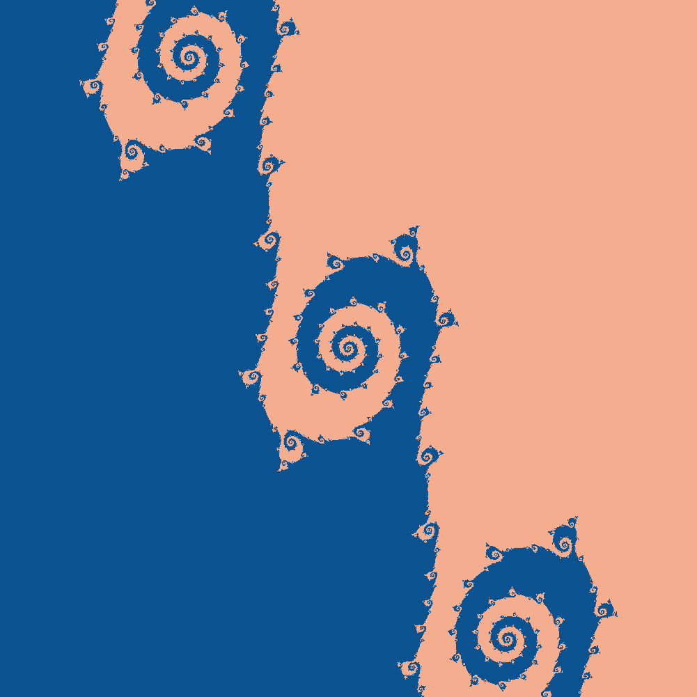
Walking around the outside edge of the boring brown circle gives a fun sequence of patterns. At there are two real fixed points and a straight line border along the imaginary axis. This line of course contains the singularity points where things get sent to infinity, and near them the preimages of all the other singularities on the line: dramatic, but visually uninteresting.
Tanh ‘Julia set’ for c=1.
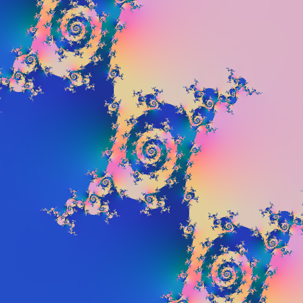
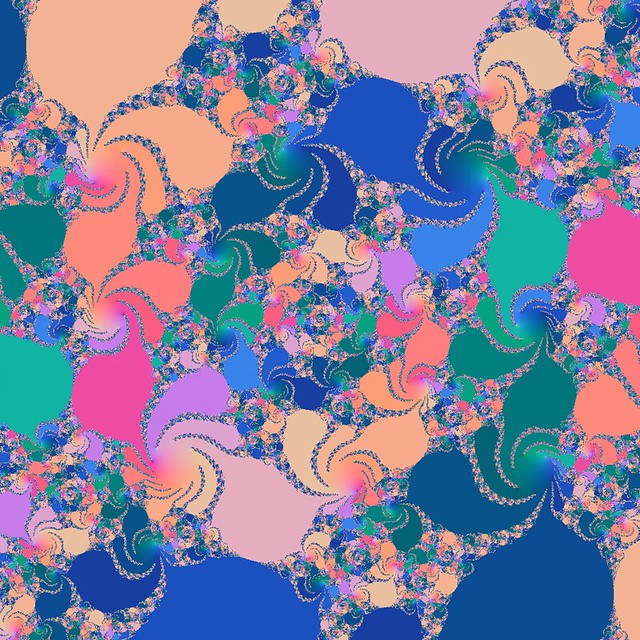
As we move along the circle towards more imaginary c, there is a twisting of the border since each multiplication by c corresponds to a twist: it is now a fractal spiral covered by little spirals. As the twisting gets stronger, the spirals get bigger and wilder (especially when we are very close to the unit circle, where the dynamics has a lot of intermittency: the iterates almost but not quite gets stuck close to certain points, speed away, and then return to make rather elliptic spirals).
Tanh ‘Julia set’ for c=1.1*exp(0.23*i).Tanh ‘Julia set’ for c=1.1*exp(0.5*i).Tanh ‘Julia set’ for c=1.1*exp(0.55*i).
When we advance towards a cuspy border in the c-plane we see the spirals unfold into long twisty tentacles just before touching, turning into borders between chains of periodic domains.
Tanh ‘Julia set’ for c=1.1*exp(0.6*i).
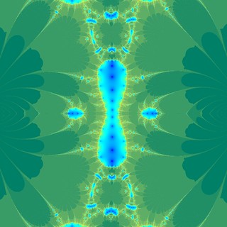
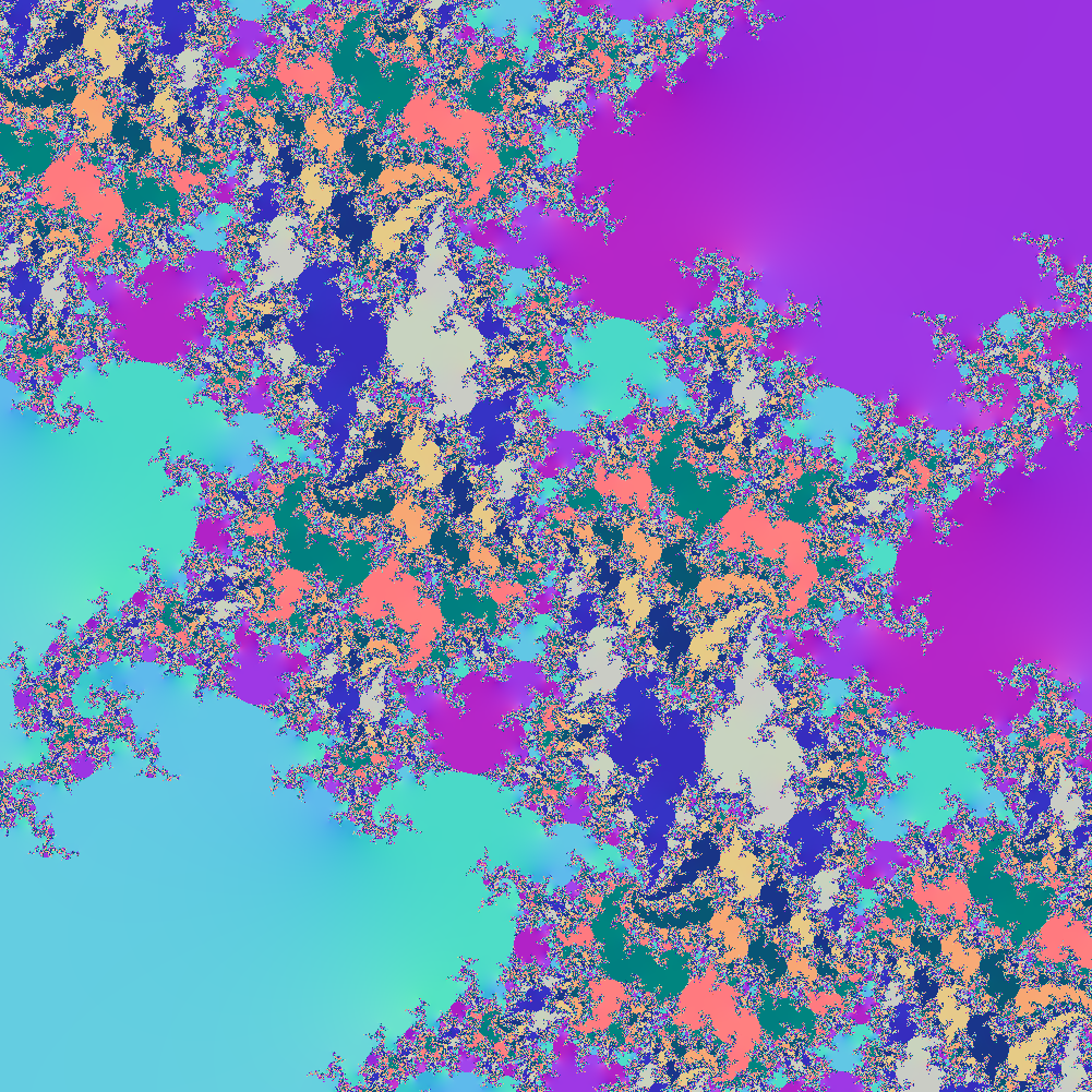
But then the periodic domains start to snake out, filling the plane wildly.
Tanh ‘Julia set’ for c=1.1*exp(0.6594*i).
until we get a plane-filling, ergodic Julia set with no discernible structure. For some c-values there are complex tesselations of basins of attraction, and quite often some places are close enough to weakly repelling fixed points to produce small circular false basins of attraction where divergence is slow.
Tanh ‘Julia set’ for c=1.1*exp(0.66*i).
One way of visualizing this is to make a bifurcation diagram like we do for real iteration. Following a curve we plot where iterates end up projected along some line (for example their real or imaginary part, or some combination). To make structure stand out a bit more I decided to color points after where in the whole plane they are, producing a colorful diagram for r=1.1:
Tanh 5.0 – r=5.0. Rather sedate except for a brief window near .
Note how spirals unfold until they touch each other, forming periodic domains or exploding across the entire plane, making a chaotic full-plane attractor… which often blinks into complex patterns of periodic domains only to return to chaos.
I like the idea of a thanksgiving day, leaving out all the Americana turkeys, problematic immigrant-native relations and family logistics: just the moment to consider what really matters to you and why life is good. And giving thanks for intellectual achievements and tools makes eminent sense: This thanksgiving Sean Carroll gave thanks for the Fourier transform.
Inspired by this, I want to give thanks for Occam’s razor.
These days a razor in philosophy denotes a rule of thumb that allows one to eliminate something unnecessary or unlikely. Occam’s was the first: William of Ockham (ca. 1285-1349) stated “Pluralitas non est ponenda sine neccesitate” (“plurality should not be posited without necessity.”) Today we usually phrase it as “the simplest theory that fits is best”.
Principles of parsimony have been suggested for a long time; Aristotle had one, so did Maimonides and various other medieval thinkers. But let’s give Bill from Ockham the name in the spirit of Stigler’s law of eponymy.
Of course, it is not always easy to use. Is the many worlds interpretation of quantum mechanics possible to shave away? It posits an infinite number of worlds that we cannot interact with… except that it does so by taking the quantum mechanics formalism seriously (each possible world is assigned a probability) and not adding extra things like wavefunction collapse or pilot waves. In many ways it is conceptually simpler: just because there are a lot of worlds doesn’t mean they are wildly different. Somebody claiming there is a spirit world is doubling the amount of stuff in the universe, but that there is a lot of ordinary worlds is not too different from the existence of a lot of planets.
Simplicity is actually quite complicated. One can argue about which theory has the fewest and most concise basic principles, but also the number of kinds of entities postulated by the theory. Not to mention why one should go for parsimony at all.
In my circles, we like to think of the principle in terms of Bayesian statistics and computational complexity. The more complex a theory is, the better it can typically fit known data – but it will also generalize worse to new data, since it overfits the first set of data points. Parsimonious theories have fewer degrees of freedom, so they cannot fit as well as complex theories, but they are less sensitive to noise and generalize better. One can operationalize the optimal balance using various statistical information criteria (AIC = minimize the information lost when fitting, BIC = maximize likeliehood of the model). And Solomonoff gave a version of the razor in theoretical computer science: for computable sequences of bits there exists a unique (up to choice of Turing machine) prior that promotes sequences generated by simple programs and has awesome powers of inference.
But in day-to-day life Occam works well, especially with a maximum probability principle (you are more likely to see likely things than unlikely; if you see hoofprints in the UK, think horses not zebras). A surprising number of people fall for the salient stories inherent in unlikely scenarios and then choose to ignore Occam (just think of conspiracy theories). If the losses from low-probability risks are great enough one should rationally focus on them, but then one must check one’s priors for such risks. Starting out with a possibilistic view that anything is possible (and hence have roughly equal chance) means that one becomes paranoid or frozen with indecision. Occam tells you to look for the simple, robust ways of reasoning about the world. When they turn out to be wrong, shift gears and come up with the next simplest thing.
Simplicity might sometimes be elegant, but that is not why we should choose it. To me it is the robustness that matters: given our biased, flawed thought processes and our limited and noisy data, we should not build too elaborate castles on those foundations.
 at the point with maximal distance
 ") from the border.
from the border.") , which is then updated
, which is then updated  \leftarrow \min(d(x,y), D(x,y))") where
where ") is the distance to the circle. This trades exactness for some discretization error, but it can easily handle nearly arbitrary shapes.
is the distance to the circle. This trades exactness for some discretization error, but it can easily handle nearly arbitrary shapes.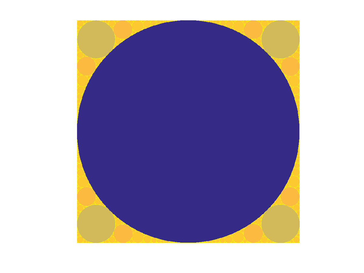
 .
.
\propto r^-\delta") as we approach zero, with
as we approach zero, with  . This is unsurprising: given a generic curved triangle, the inscribed circle will be a fraction of the radii of the bordering circles. If one looks at
  is the Hausdorff dimension of the gasket.
 .
.
 we get sponge-like fractals: these are relatives to the Menger sponge and the Cantor set. The domain gets an infinity of circles punched out of itself, with a total area approaching the area of the domain, so the total measure goes to zero.

 random samples, the posterior distribution of
  , the number of pages, is
  = P(k|N)P(N)/P(k)") .
. , on my third try
  , and so on:
 =(k-1)/N") . Of course, there has to be more pages than
. Of course, there has to be more pages than  , otherwise a repeat must have happened before step
  . Otherwise,
 =0") for
for  .
.") needs to be decided. One approach is to assume that websites have
needs to be decided. One approach is to assume that websites have  = N^{-\alpha}/\zeta(\alpha)") . Note the appearance of the Riemann zeta function as a normalisation factor.
. Note the appearance of the Riemann zeta function as a normalisation factor.") by summing over the different possible
by summing over the different possible =\sum_{N=1}^\infty P(k|N)P(N) = \frac{k-1}{\zeta(\alpha)}\sum_{N=k-1}^\infty N^{-(\alpha+1)}")
}(\zeta(\alpha+1)-\sum_{i=1}^{k-2}i^{-(\alpha+1)})") .
.=N^{-(\alpha+1)}/(\zeta(\alpha+1) -\sum_{i=1}^{k-2}i^{-(\alpha+1)})") for
for  . The posterior distribution of number of pages is another power-law. Note that the dependency on
 =\sum_{N=1}^\infty N P(N|k) = \sum_{N=k-1}^\infty N^{-\alpha}/(\zeta(\alpha+1) -\sum_{i=1}^{k-2}i^{-(\alpha+1)})")
-\sum_{i=1}^{k-2} i^{-\alpha}}{\zeta(\alpha+1)-\sum_{i=1}^{k-2}i^{-(\alpha+1)}}") . The expectation is the ratio of the zeta functions of
. The expectation is the ratio of the zeta functions of  , minus the first
  terms of their series.
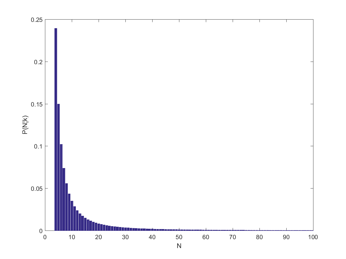
 (close to the behavior of big websites), it predicts
 \approx 21.28") . If one assumes a higher
. If one assumes a higher  the number of pages would be 7 (which was close to the size of the wiki when I looked at it last night – it has grown enough today for k to equal 13 when I tried it today).
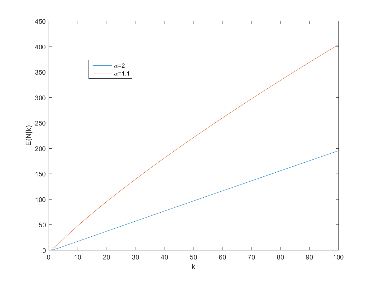
") approaches proportionality, especially for larger
approaches proportionality, especially for larger 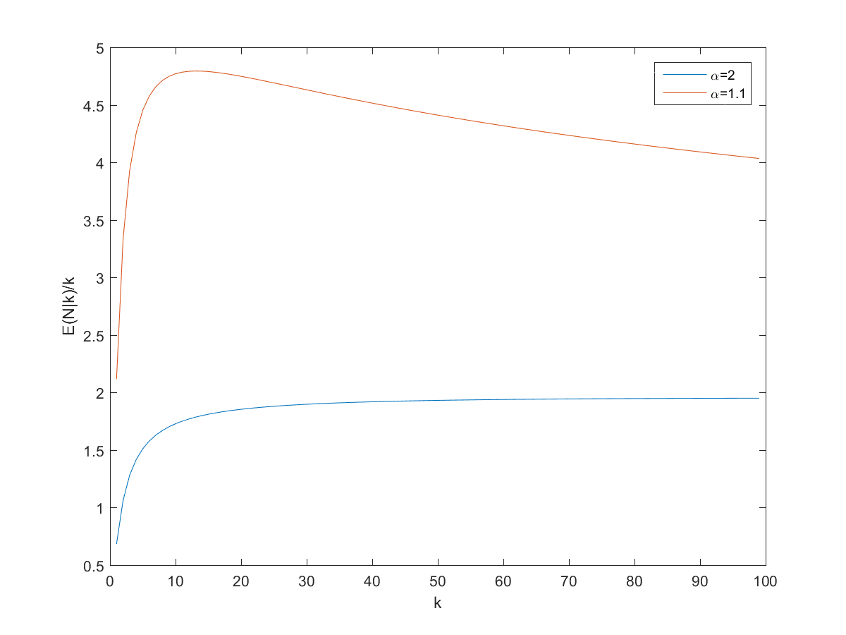
 and
and  pages on the site. However, remember that we are dealing with power-laws, so the variance can be surprisingly high.

 .
.dx\right)dx\right)dx") .
. , the x in the second will be integrated twice
  , and so on.
=\int f(x)+\left(\int f(x)+\left(\int f(x)+\left(\ldots\right)dx\right)dx\right)dx = \sum_{n=1}^\infty \int^n f(x) dx") .
.=f(x)+I(x)") .
.=\sin(kx)") we get the sum
we get the sum =-\cos(kx)/k-\sin(kx)/k^2+\cos(kx)/k^3+\sin(x)/k^4-\cos(kx)/k^5-\ldots") . For
. For  we end up with
 =\sum_{n=0}^\infty 1/k^{4n+2} - \sum_{n=0}^\infty 2/k^{4n+1}") . The differential equation has solution
. The differential equation has solution =ce^x-\sin(kx)/(k^2+1) - k\cos(kx)/(k^2+1)") . Setting
. Setting  the integral is clearly zero, so
  . Tying it together we get:
") .
.=\int x \int x \int x \ldots dx dx dx") . However, we can turn it into a differential equation:
. However, we can turn it into a differential equation: =x I(x)") which has the well known solution
which has the well known solution =ce^{x^2/2}") . Same thing for
. Same thing for =ce^{-\cos(kx)/k}") . Since we are running indefinite integrals we get those pesky constants.
. Since we are running indefinite integrals we get those pesky constants.=1/x") gives
gives =cx") . If we set
. If we set  we get the mildly amusing and in retrospect obvious formula
 .
.=\int\sqrt{\int\sqrt{\int\sqrt{\ldots} dx} dx} dx") , where the differential equation becomes
, where the differential equation becomes  with the solution
 =(1/4)(c^2 + 2cx + x^2)") . A surprisingly simple solution to a weird-looking integral. In a similar vein:
. A surprisingly simple solution to a weird-looking integral. In a similar vein:=\int\sin\left(\int\sin\left(\int\sin\left(\ldots\right)dx\right) dx\right) dx")
=\int \exp\left(\int \exp\left(\int \exp\left(\ldots \right) dx \right) dx \right) dx")
=\int \left(\int \left(\int \left(\ldots \right)^2 dx \right)^2 dx \right)^2 dx")
=\int W\left(\int W\left(\int W\left(\ldots \right) dx \right) dx \right) dx") , then
, then }1/W(t) dt + c") .
. is holomorphic, then
=\Re\left(\int_{z_0}^z f(1-g^2)/2 dz\right)")
=\Re\left(\int_{z_0}^z if(1+g^2)/2 dz\right)")
=\Re\left(\int_{z_0}^z fg dz\right)")
,Y(z),Z(z))") .
.") .
. to different points
  in the complex plane. Let us start with the simple case of
 >1/2") .
.
 – a rather neat residue!) to the coordinates: a translation in the positive y-direction. If we extend the surface by going an extra turn clockwise or counterclockwise a number of times, we get copies that attach seamlessly.
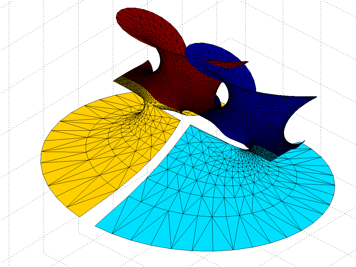
 . They also introduce residues along the y-direction, but different ones from the z=0 – their extensions of the surface will be out of phase with each other, making the fully extended surface fantastically self-intersecting and confusing.
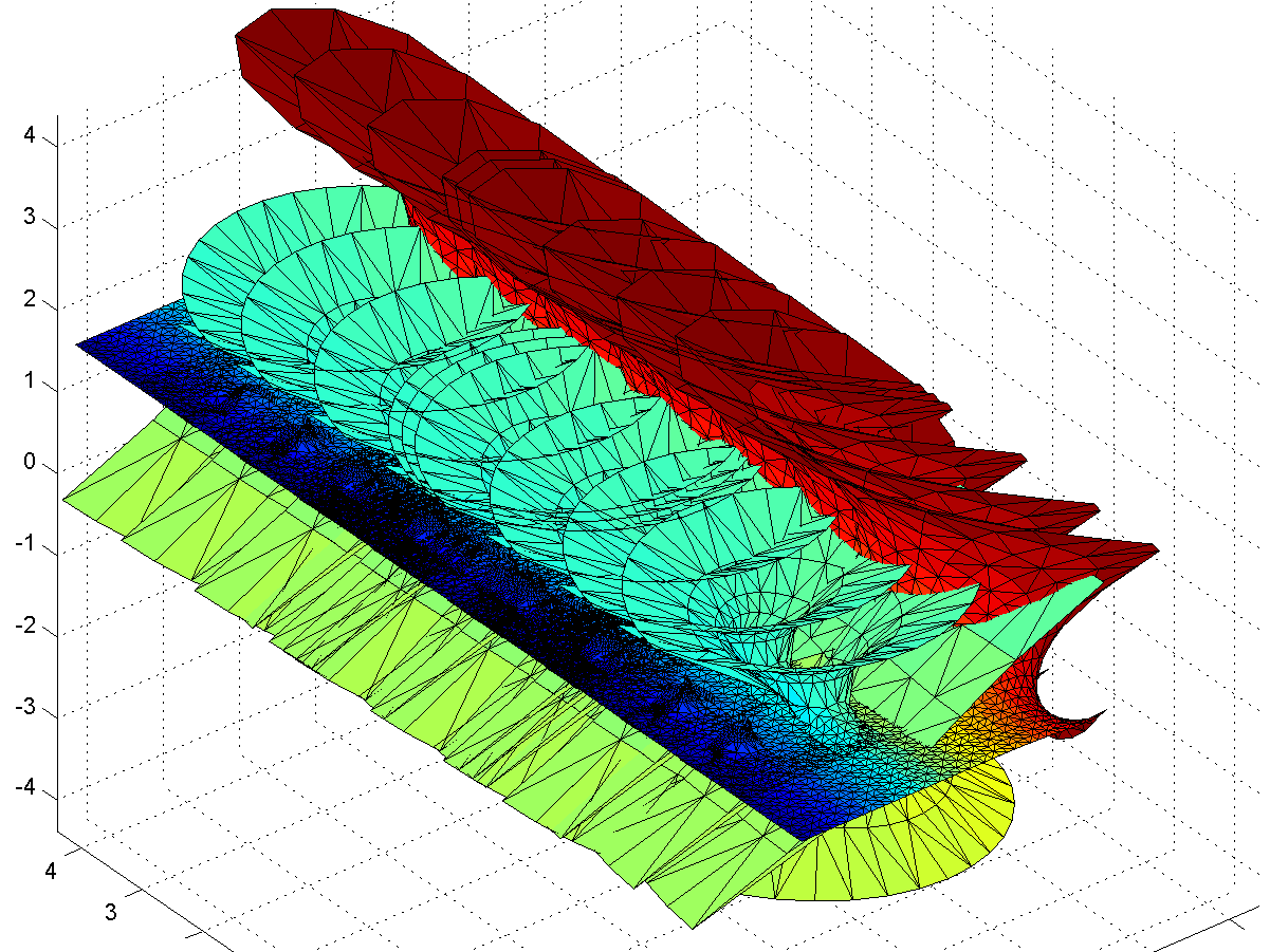
") is nicely behaved and looks very much like the Enneper surface near zero, with “wings” that oscillate ever more wildly as we move towards the negative reals. No doubt there are other beautiful things to look for in the vicinity.
is nicely behaved and looks very much like the Enneper surface near zero, with “wings” that oscillate ever more wildly as we move towards the negative reals. No doubt there are other beautiful things to look for in the vicinity.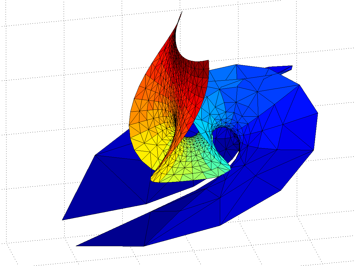
=\int_0^\infty t^{z-1}e^{-t} dt") , the continuous generalization of the factorial. While it grows rapidly for positive reals, it has fun poles for the negative integers and is generally complex.
, the continuous generalization of the factorial. While it grows rapidly for positive reals, it has fun poles for the negative integers and is generally complex. ") . The result is a nice fractal, with some domains approaching 1, and others running off to infinity.
. The result is a nice fractal, with some domains approaching 1, and others running off to infinity.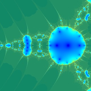
 . Zooming in a bit more reveals neat self-similar patterns with alternating “beans”:
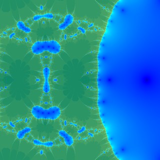
") where c is the control parameter. I start with
where c is the control parameter. I start with 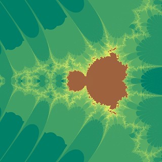
 has an infinite decimal expansion, does that mean the collected works of Shakespeare (suitably encoded) are in it somewhere?”
 is a Shakespeare-free number (unless we have a bizarre encoding of the works in the form of all threes). What really matters is whether the number is suitably random. In mathematics this is known as the question about whether pi is a
 ![[Shakespeare]](http://s0.wp.com/latex.php?latex=%5BShakespeare%5D&bg=ffffff&fg=000000&s=0 "[Shakespeare]") , all numbers of the form
, all numbers of the form ![0.[Shakespeare]xxxxx\ldots](http://s0.wp.com/latex.php?latex=0.%5BShakespeare%5Dxxxxx%5Cldots+&bg=ffffff&fg=000000&s=0 "0.[Shakespeare]xxxxx\ldots") are Shakespeare-containing.
are Shakespeare-containing.![[0. 527269000\ldots , 0.52727]](http://s0.wp.com/latex.php?latex=%5B0.+527269000%5Cldots+%2C+0.52727%5D&bg=ffffff&fg=000000&s=0 "[0. 527269000\ldots , 0.52727]") , a mere millionth of
, a mere millionth of ![[0,1]](http://s0.wp.com/latex.php?latex=%5B0%2C1%5D&bg=ffffff&fg=000000&s=0 "[0,1]") . The actual interval is even shorter.
. The actual interval is even shorter.![0.y[Shakespeare]xxxx\ldots](http://s0.wp.com/latex.php?latex=0.y%5BShakespeare%5Dxxxx%5Cldots+&bg=ffffff&fg=000000&s=0 "0.y[Shakespeare]xxxx\ldots") , where
, where  is a digit different from the starting digit of
  anything else. So there are 9 such second level intervals, each ten times thinner than the first level interval.
![[Shakespeare]=3](http://s0.wp.com/latex.php?latex=%5BShakespeare%5D%3D3&bg=ffffff&fg=000000&s=0 "[Shakespeare]=3") , so all numbers containing the digit 3 in the decimal expansion are Shakespearian and the rest are Shakespeare-free.
, so all numbers containing the digit 3 in the decimal expansion are Shakespearian and the rest are Shakespeare-free.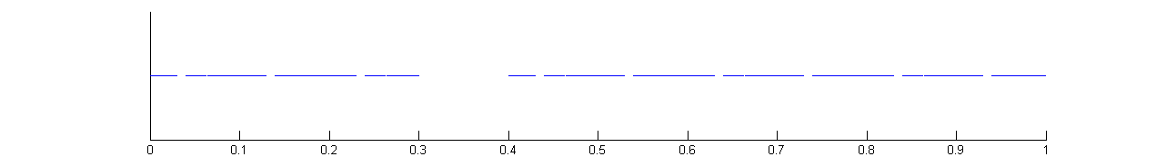
/\log(10)\approx 0.9542") . This is less than 1: most points are Shakespearian and in one of the intervals, but since they are thin compared to the line the Shakespeare-free set is nearly one dimensional. Like the Cantor set, each Shakespeare-free number is isolated from any other Shakespeare-free number: there is always some Shakespearian numbers between them.
. This is less than 1: most points are Shakespearian and in one of the intervals, but since they are thin compared to the line the Shakespeare-free set is nearly one dimensional. Like the Cantor set, each Shakespeare-free number is isolated from any other Shakespeare-free number: there is always some Shakespearian numbers between them. . The fractal dimension of the Shakespeare-free set is
 /\log(10^{10,600,600}) \approx 1-\epsilon") , for some tiny
, for some tiny  . It is very nearly an unbroken line… except for that nearly every point actually does contain Shakespeare.
![[Shakespeare][Shakespeare]xxx\ldots](http://s0.wp.com/latex.php?latex=%5BShakespeare%5D%5BShakespeare%5Dxxx%5Cldots&bg=ffffff&fg=000000&s=0 "[Shakespeare][Shakespeare]xxx\ldots") numbers…
numbers… of being in the level 1 interval of Shakespearian numbers. If not, then it will be in one of the 9 intervals 1/10 long that don’t start with the correct first digit, where the probability of starting with Shakespeare in the second digit is
 S+(9/10^2)S+\ldots = 10S<1") . But the 1/10 interval around the first Shakespearian interval also counts: a number that has the right first digit but wrong second digit can still be Shakespearian. So it will add probability.
. But the 1/10 interval around the first Shakespearian interval also counts: a number that has the right first digit but wrong second digit can still be Shakespearian. So it will add probability.S") (the first factor is the probability of not having Shakespeare first), and so on. So the total probability of finding Shakespeare is
(the first factor is the probability of not having Shakespeare first), and so on. So the total probability of finding Shakespeare is S + (1-S)^2S + (1-S)^3S + \ldots = S/(1-(1-S))=1") . So nearly all numbers are Shakespearian.
. So nearly all numbers are Shakespearian.![0.[Shakespeare]000\ldots](http://s0.wp.com/latex.php?latex=0.%5BShakespeare%5D000%5Cldots+&bg=ffffff&fg=000000&s=0 "0.[Shakespeare]000\ldots") is non-normal but Shakespearian. So is
is non-normal but Shakespearian. So is ![0.[Shakespeare][Shakespeare][Shakespeare]\ldots](http://s0.wp.com/latex.php?latex=0.%5BShakespeare%5D%5BShakespeare%5D%5BShakespeare%5D%5Cldots+&bg=ffffff&fg=000000&s=0 "0.[Shakespeare][Shakespeare][Shakespeare]\ldots") We can throw in arbitrary finite sequences of digits between the Shakespeares, biasing numbers as close or far as we want from normality. There is a number
We can throw in arbitrary finite sequences of digits between the Shakespeares, biasing numbers as close or far as we want from normality. There is a number ![0.[Shakespeare]3141592\ldots](http://s0.wp.com/latex.php?latex=0.%5BShakespeare%5D3141592%5Cldots&bg=ffffff&fg=000000&s=0 "0.[Shakespeare]3141592\ldots") that has the digits of
that has the digits of 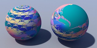
 = \tanh(cz_n)") , where c is a multiplicative constant. Iterating some number like 1 and plotting its fate produces the following “Mandelbrot set” in the c-plane – the colours here do not denote the time until escape to infinity but rather where in the complex plane the point ended up, as a function of c. In a normal Mandelbrot set infinity is an attractive fixed point; here it is just one place in the (extended) complex plane like any other.
, where c is a multiplicative constant. Iterating some number like 1 and plotting its fate produces the following “Mandelbrot set” in the c-plane – the colours here do not denote the time until escape to infinity but rather where in the complex plane the point ended up, as a function of c. In a normal Mandelbrot set infinity is an attractive fixed point; here it is just one place in the (extended) complex plane like any other.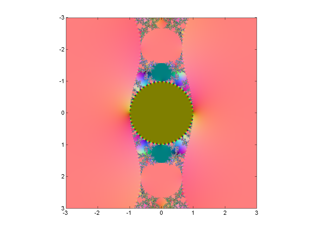
") . There is of course a corresponding negative solution since tanh is antisymmetric: if z is an attractive fixed point or cycle, so is -z. So the dynamics is always bistable.
. There is of course a corresponding negative solution since tanh is antisymmetric: if z is an attractive fixed point or cycle, so is -z. So the dynamics is always bistable.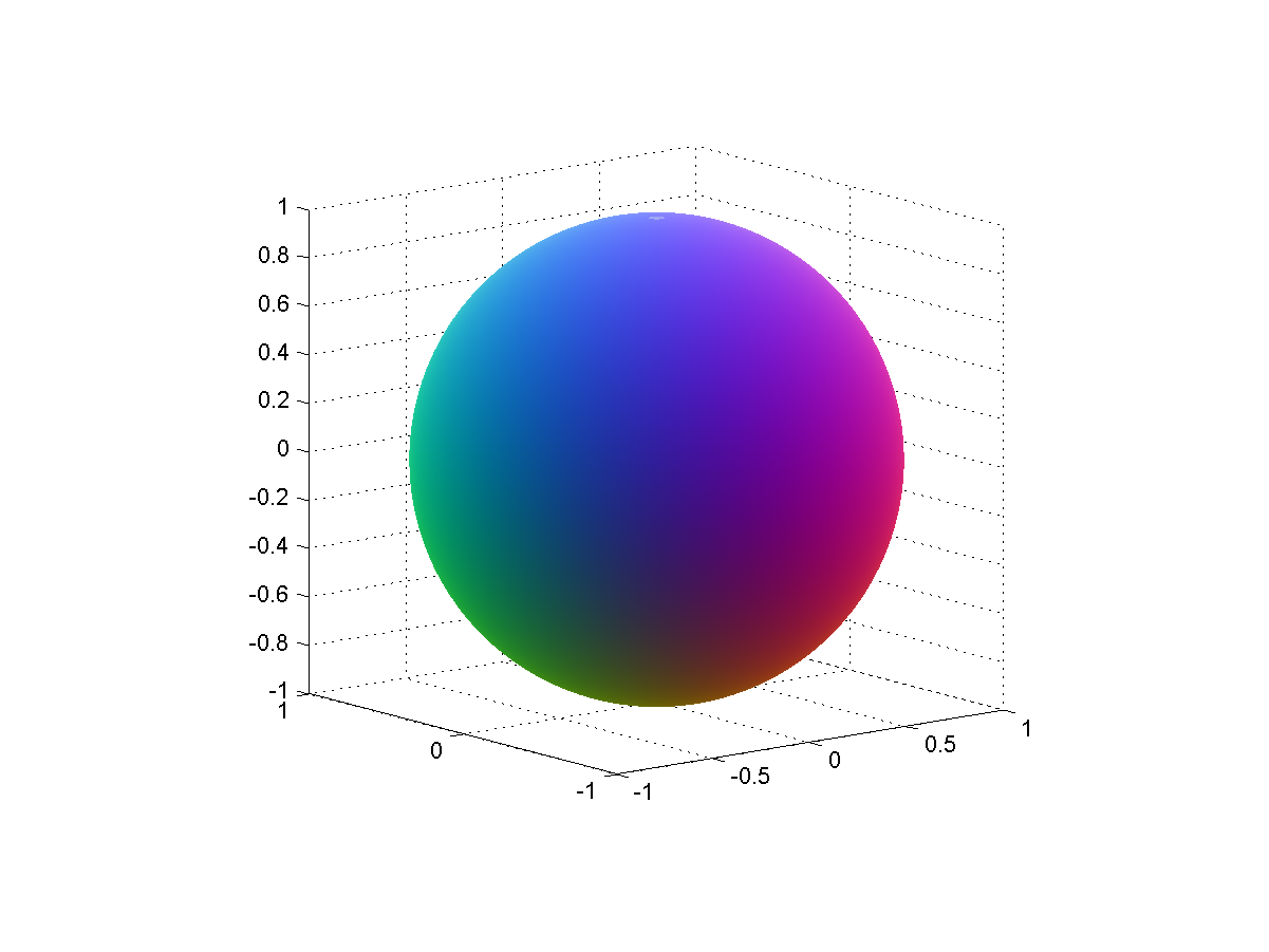
 for integer
  . Since


 we plot where iterates end up projected along some line (for example their real or imaginary part, or some combination). To make structure stand out a bit more I decided to color points after where in the whole plane they are, producing a colorful diagram for r=1.1:
 is at the center, zero outside the borders.
 .
.
