Review of the cyborg bill of rights 1.0

The Cyborg Bill of Rights 1.0 is out. Rich MacKinnon suggests the following rights:

FREEDOM FROM DISASSEMBLY
A person shall enjoy the sanctity of bodily integrity and be free from unnecessary search, seizure, suspension or interruption of function, detachment, dismantling, or disassembly without due process.

FREEDOM OF MORPHOLOGY
A person shall be free (speech clause) to express themselves through temporary or permanent adaptions, alterations, modifications, or augmentations to the shape or form of their bodies. Similarly, a person shall be free from coerced or otherwise involuntary morphological changes.

RIGHT TO ORGANIC NATURALIZATION
A person shall be free from exploitive or injurious 3rd party ownerships of vital and supporting bodily systems. A person is entitled to the reasonable accrual of ownership interest in 3rd party properties affixed, attached, embedded, implanted, injected, infused, or otherwise permanently integrated with a person’s body for a long-term purpose.

RIGHT TO BODILY SOVEREIGNTY
A person is entitled to dominion over intelligences and agents, and their activities, whether they are acting as permanent residents, visitors, registered aliens, trespassers, insurgents, or invaders within the person’s body and its domain.

EQUALITY FOR MUTANTS
A legally recognized mutant shall enjoy all the rights, benefits, and responsibilities extended to natural persons.

As a sometime philosopher with a bit of history of talking about rights regarding bodily modification, I of course feel compelled to comment.

What are rights?

First, what is a right? Clearly anybody can state that we have a right to X, but only some agents and X-rights make sense or have staying power.

One kind of rights are legal rights of various kinds. This can be international law, national law, or even informal national codes (for example the Swedish allemansrätten, which is actually not a moral/human right and actually fairly recent). Here the agent has to be some legitimate law- or rule-maker. The US Bill of Rights is an example: the result of a political process that produced legal rights, with relatively little if any moral content. Legal rights need to be enforceable somehow.

Then there are normative moral principles such as fundamental rights (applicable to a person since they are a person), natural rights (applicable because of facts of the world) or divine rights (imposed by God). These are universal and egalitarian: applicable everywhere, everywhen, and the same for everybody. Bentham famously dismissed the idea of natural rights as “nonsense on stilts” and there is a general skepticism today about rights being fundamental norms. But insofar they do exist, anybody can discover and state them. Moral rights need to be doable.

While there may be doubts about the metaphysical nature of rights, if a society agrees on a right it will shape action, rules and thinking in an important way. It is like money: it only gets value by the implicit agreement that it has value and can be exchanged for goods. Socially constructed rights can be proposed by anybody, but they only become real if enough people buy into the construction. They might be unenforceable and impossible to perform (which may over time doom them).

What about the cyborg rights? There is no clear reference to moral principles, and only the last one refers to law. In fact, the preamble states:

Our process begins with a draft of proposed rights that are discussed thoroughly, adopted by convention, and then published to serve as model language for adoption and incorporation by NGOs, governments, and rights organizations.

That is, these rights are at present a proposal for social construction (quite literally) that hopefully will be turned into a convention (a weak international treaty) that eventually may become national law. This also fits with the proposal coming from MacKinnon rather than the General Secretary of the UN – we can all propose social constructions and urge the creation of conventions, treaties and laws.

But a key challenge is to come up with something that can become enforceable at some point. Cyborg bodies might be more finely divisible and transparent than human bodies, so that it becomes hard to regulate these rights. How do you enforce sovereignty against spyware?

Justification

Why is a right a right? There has to be a reason for a right (typically hinted at in preambles full of “whereas…”)

I have mostly been interested in moral rights. Patrick D. Hopkins wrote an excellent overview “Is enhancement worthy of being a right?” in 2008 where he looks at how you could motivate morphological freedom. He argues that there are three main strategies to show that a right is fundamental or natural:

That the right conforms to human nature. This requires showing that it fits a natural end. That is, there are certain things humans should aim for, and rights help us live such lives. This is also the approach of natural law accounts.
That the right is grounded in interests. Rights help us get the kinds of experiences or states of the world that we (rightly) care about. That is, there are certain things that are good for us (e.g. “the preservation of life, health, bodily integrity, play, friendship, classic autonomy, religion, aesthetics, and the pursuit of knowledge”) and the right helps us achieve this. Why those things are good for us is another matter of justification, but if we agree on the laundry list then the right follows if it helps achieve them.
That the right is grounded in our autonomy. The key thing is not what we choose but that we get to choose: without freedom of choice we are not moral agents. Much of rights by this account will be about preventing others from restricting our choices and not interfering with their choices. If something can be chosen freely and does not harm others, it has a good chance to be a right. However, this is a pretty shallow approach to autonomy; there are more rigorous and demanding ideas of autonomy in ethics (see SEP and IEP for more). This is typically how many fundamental rights get argued (I have a right to my body since if somebody can interfere with my body, they can essentially control me and prevent my autonomy).

One can do this in many ways. For example, David Miller writes on grounding human rights that one approach is to allow people from different cultures to live together as equals, or basing rights on human needs (very similar to interest accounts), or the instrumental use of them to safeguard other (need-based) rights. Many like to include human dignity, another tricky concept.

Social constructions can have a lot of reasons. Somebody wanted something, and this was recognized by others for some reason. Certain reasons are cultural universals, and that make it more likely that society will recognize a right. For example, property seems to be universal, and hence a right to one’s property is easier to argue than a right to paid holidays (but what property is, and what rules surround it, can be very different).

Legal rights are easier. They exist because there is a law or treaty, and the reasons for that are typically a political agreement on something.

It should be noted that many declarations of rights do not give any reasons. Often because we would disagree on the reasons, even if we agree on the rights. The UN declaration of human rights give no hint of where these rights come from (compare to the US declaration of independence, where it is “self-evident” that the creator has provided certain rights to all men). Still, this is somewhat unsatisfactory and leaves many questions unanswered.

So, how do we justify cyborg rights?

In the liberal rights framework I used for morphological freedom we could derive things rather straightforwardly: we have a fundamental right to life, and from this follows freedom from disassembly. We have a fundamental right to liberty, and together with the right to life this leads to a right to our own bodies, bodily sovereignty, freedom of morphology and the first half of the right to organic naturalization. We have a right to our property (typically derived from fundamental rights to seek our happiness and have liberty), and from this the second half of the organic naturalization right follows (we are literally mixing ourselves rather than our work with the value produced by the implants). Equality for mutants follow from having the same fundamental rights as humans (note that the bill talks about “persons”, and most ethical arguments try to be valid for whatever entities count as persons – this tends to be more than general enough to cover cyborg bodies). We still need some justification of the fundamental rights of life, liberty and happiness, but that is outside the scope of this exercise. Just use your favorite justifications.

The human nature approach would say that cyborg nature is such that these rights fit with it. This might be tricky to use as long as we do not have many cyborgs to study the nature of. In fact, since cyborgs are imagined as self-creating (or at least self-modifying) beings it might be hard to find any shared nature… except maybe the self-creation part. As I often like to argue, this is close to Mirandola’s idea of human dignity deriving from our ability to change ourselves.

The interest approach would ask how the cyborg interests are furthered by these rights. That seems pretty straightforward for most reasonably human-like interests. In fact, the above liberal rights framework is to a large extent an interest-based account.

The autonomy account is also pretty straightforward. All cyborg rights except the last are about autonomy.

Could we skip the ethics and these possibly empty constructions? Perhaps: we could see the cyborg bill of rights as a way of making a cyborg-human society possible to live in. We need to tolerate each other and set boundaries on allowed messing around with each other’s bodies. Universals of property lead to the naturalization right, territoriality the sovereignty right universal that actions under self-control are distinguished from those not under control might be taken as the root for autonomy-like motivations that then support the rest.

Which one is best? That depends. The liberal rights/interest system produces nice modular rules, although there will be much arguments on what has precedence. The human nature approach might be deep and poetic, but potentially easy to disagree on. Autonomy is very straightforward (except when the cyborg starts messing with their brain). Social constructivism allows us to bring in issues of what actually works in a real society, not just what perfect isolated cyborgs (on a frictionless infinite plane) should do.

Parts of rights

One of the cool properties of rights is that they have parts – “the Hohfeldian incidents“, after Wesley Hohfeld (1879–1918) who discovered them. He was thinking of legal rights, but this applies to moral rights too. His system is descriptive – this is how rights work – rather than explaining why the came about or whether this is a good thing. The four parts are:

Privileges (alias liberties): I have a right to eat what I want. Someone with a driver’s licence has the privilege to drive. If you have a duty not do do something, then you have no privilege about it.

Claims: I have a claim on my employer to pay my salary. Children have a claim vis-a-vis every adult not to be abused. My employer is morally and legally dutybound to pay, since they agreed to do so. We are dutybound to refrain from abusing children since it is wrong and illegal.

These two are what most talk about rights deal. In the bill, the freedom from disassembly and freedom of morphology are about privileges and claims. The next two are a bit meta, dealing with rights over the first two:

Powers: My boss has the power to order me to research a certain topic, and then I have a duty to do it. I can invite somebody to my home, and then they have the privilege of being there as long as I give it to them. Powers allow us to change privileges and claims, and sometimes powers (an admiral can relieve a captain of the power to command a ship).

Immunities: My boss cannot order me to eat meat. The US government cannot impose religious duties on citizens. These are immunities: certain people or institutions cannot change other incidents.

These parts are then combined into full rights. For example, my property rights to this computer involve the privilege to use the computer, a claim against others to not use the computer, the power to allow others to use it or to sell it to them (giving them the entire rights bundle), and an immunity of others altering these rights. Sure, in practice the software inside is of doubtful loyalty and there are law-enforcement and emergency situation exceptions, but the basic system is pretty clear. Licence agreements typically give you a far

Sometimes we speak about positive and negative rights: if I have a negative right I am entitled to non-interference from others, while a positive right entitles me to some help or goods. My right to my body is a negative right in the sense that others may not prevent me from using or changing my body as I wish, but I do not have a positive right to demand that they help me with some weird bodymorphing. However, in practice there is a lot of blending going on: public healthcare systems give us positive rights to some (but not all) treatment, policing gives us a positive right of protection (whether we want it or not). If you are a libertarian you will tend to emphasize the negative rights as being the most important, while social democrats tend to emphasize state-supported positive rights.

The cyborg bill of rights starts by talking about privileges and claims. Freedom of morphology clearly expresses an immunity to forced bodily change. The naturalization right is about immunity from unwilling change of the rights of parts, and an expression of a kind of power over parts being integrated into the body. Sovereignty is all about power over entities getting into the body.

The right of bodily sovereignty seems to imply odd things about consensual sex – once there is penetration, there is dominion. And what about entities that are partially inside the body? I think this is because it is trying to reinvent some of the above incidents. The aim is presumably to cover pregnancy/abortion, what doctors may do, and other interventions at the same time. The doctor case is easy, since it is roughly what we agree on today: we have the power to allow doctors to work on our bodies, but we can also withdraw this whenever we want

Some other thoughts

The recent case where the police subpoenad the pacemaker data of a suspected arsonist brings some of these rights into relief. The subpoena occurred with due process, so it was allowed by the freedom from disassembly. In fact, since it is only information and that it is copied one can argue that there was no real “disassembly”. There have been cases where police wanted bullets lodged in people in order to do ballistics on them, but US courts have generally found that bodily integrity trumps the need for evidence. Maybe one could argue for a derived right to bodily privacy, but social needs can presumably trump this just as it trumps normal privacy. Right now views on bodily integrity and privacy are still based on the assumption that bodies are integral and opaque. In a cyborg world this is no longer true, and the law may well move in a more invasive direction.

“Legally recognized mutant”? What about mutants denied legal recognition? Legal recognition makes sense for things that the law must differentiate between, not for things the law is blind to. Legally recognized mutants (whatever they are) would be a group that needs to be treated in some special way. If they are just like natural humans they do not need special recognition. We may have laws making it illegal to discriminate against mutants, but this is a law about a certain kind of behavior rather than the recipient. If I racially discriminate against somebody but happens to be wrong about their race, I am still guilty. So the legal recognition part does not do any work in this right.

And why just mutants? Presumably the aim here is to cover cyborgs, transhumans and other prefix-humans so they are recognized as legal and moral agents with the same standing. The issue is whether this is achieved by arguing that they were human and “mutated”, or are descended from humans, and hence should have the same standing, or whether this is due to them having the right kind of mental states to be persons. The first approach is really problematic: anencephalic infants are mutants but hardly persons, and basing rights on lineage seems ripe for abuse. The second is much simpler, and allows us to generalize to other beings like brain emulations, aliens, hypothetical intelligent moral animals, or the Swampman.

This links to a question that might deserve a section on its own: who are the rightsholders? Normal human rights typically deal with persons, which at least includes adults capable of moral thinking and acting (they are moral agents). Someone who is incapable, for example due to insanity or being a child, have reduced rights but are still a moral patient (someone we have duties towards). A child may not have full privileges and powers, but they do have claims and immunities. I like to argue that once you can comprehend and make use of a right you deserve to have it, since you have capacity relative to the right. Some people also think prepersons like fertilized eggs are persons and have rights; I think this does not make much sense since they lack any form of mind, but others think that having the potential for a future mind is enough to grant immunity. Tricky border cases like persistent vegetative states, cryonics patients, great apes and weird neurological states keep bioethicists busy.

In the cyborg case the issue is what properties make something a potential rightsholder and how to delineate the border of the being. I would argue that if you have a moral agent system it is a rightsholder no matter what it is made of. That is fine, except that cyborgs might have interchangeable parts: if cyborg A gives her arm to cyborg B, have anything changed? I would argue that the arm switched from being a part of/property of A to being a part of/property of B, but the individuals did not change since the parts that make them moral agents are unchanged (this is just how transplants don’t change identity). But what if A gave part of her brain to B? A turns into A’, B turns into B’, and these may be new agents. Or what if A has outsourced a lot of her mind to external systems running in the cloud or in B’s brain? We may still argue that rights adhere to being a moral agent and person rather than being the same person or a person that can easily be separated from other persons or infrastructure. But clearly we can make things really complicated through overlapping bodies and minds.

Summary

I have looked at the cyborg bill of rights and how it fits with rights in law, society and ethics. Overall it is a first stab at establishing social conventions for enhanced, modular people. It likely needs a lot of tightening up to work, and people need to actually understand and care about its contents for it to have any chance of becoming something legally or socially “real”. From an ethical standpoint one can motivate the bill in a lot of ways; for maximum acceptance one needs to use a wide and general set of motivations, but these will lead to trouble when we try to implement things practically since they give no way of trading one off against another one in a principled way. There is a fair bit of work needed to refine the incidences of the rights, not to mention who is a rightsholder (and why). That will be fun.

Infinite Newton

Apropos Newton’s method in the complex plane, what happens when the degree of the polynomial goes to infinity?

Towards infinity

Obviously there will be more zeros, so there will be more attractors and we should expect the boundaries of the basins of attraction to become messier. But it is not entirely clear where the action will be, so it would be useful to compress the entire complex plane into a convenient square.

How do you depict the entire complex plane? While I have always liked the Riemann sphere here I tried mapping $x+yi$ to $[\tanh(x),\tanh(y)]$ . The origin is unchanged, and infinity becomes the edges of the square $[-1,1]\times [-1,1]$ . This is not a conformal map, so things will get squished near the edges.

For color, I used $(1/2)+(1/2)[\tanh(|z-1|-1), \tanh(|z+1|-1), \tanh(|z-i|-1)]$ to map complex coordinates to RGB. This makes the color depend on the distance to 1, -1 and i, making infinity white and zero some drab color (the -1 terms at the end determines the overall color range).

Here is the animated result:

What is going on? As I scale up the size of the leading term from zero, the root created by adding that term moves in from infinity towards the center, making the new basin of attraction grow. This behavior has been described in this post on dancing zeros. The zeros also tend to cluster towards the unit circle, crowding together and distributing themselves evenly. That distribution is the reason for the the colorful “flowers” that surround white spots (poles of the Newton formula, corresponding to zeros of the derivative of the polynomial). The central blob is just the attractor of the most “solid” zero, corresponding to the linear and constant terms of the polynomial.

The jostling is amusing: it looks like the roots do repel each other. This is presumably because close roots require a sharp turn of the function, but the “turning radius” is set by the coefficients that tend to be of order unity. Getting degenerate roots requires coefficients to be in a set of measure zero, so it is rare. Near-degenerate roots exist in a positive measure set surrounding that set, but it is still “small” compared to the general case.

At infinity

So what happens if we let the degree go to infinity? As I previously mentioned, the generic behaviour of $\sum_{n=1}^\infty a_n z^n$ where $a_n$ is independent random numbers is a lacunary function. So we should not expect anything outside the unit circle. Inside the circle there will be poles, so there will be copies of the undefined outside region (because of Great Picard’s Theorem (meromorphic version)). Since the function is analytic these copies will be conformal mappings of the exterior and hence roughly circular. There will also be zeros, and these will have their own basins of attraction. A few of the central ones dominate, but there is an infinite number of attractors as we approach the circular border which is crammed with poles and zeros.

Since we now know we will only deal with the unit disk, we can avoid transforming the entire plane and enjoy the results:

Attractors for random 10,000-degree polynomial.

What happens here is that the white regions represents places where points get mapped onto the undefined outside, while the colored fractal regions are the attraction basins for the zeros. And between them there is a truly wild boundary. In the vanilla $z^3+1$ fractal every point on the boundary is a meeting point of the three basins, a tri-point. Here there is an infinite number of attractors: the boundary consists of points where an infinite number of different attractors meet.

Checking my predictions for 2016

Last year I made a number of predictions for 2016 to see how well calibrated I am. Here is the results:

Prediction	Correct?
No nuclear war: 99%	1
No terrorist attack in the USA will kill > 100 people: 95%	1 (Orlando: 50)
I will be involved in at least one published/accepted-to-publish research paper by the end of 2015: 95%	1
Vesuvius will not have a major eruption: 95%	1
I will remain at my same job through the end of 2015: 90%	1
MAX IV in Lund delivers X-rays: 90%	1
Andart II will remain active: 90%	1
Israel will not get in a large-scale war (ie >100 Israeli deaths) with any Arab state: 90%	1
US will not get involved in any new major war with death toll of > 100 US soldiers: 90%	1
New Zeeland has not decided to change current flag at end of year: 85%	1
No multi-country Ebola outbreak: 80%	1
Assad will remain President of Syria: 80%	1
ISIS will control less territory than it does right now: 80%	1
North Korea’s government will survive the year without large civil war/revolt: 80%	1
The US NSABB will allow gain of function funding: 80%	1 [Their report suggests review before funding, currently it is up to the White House to respond. ]
US presidential election: democratic win: 75%	0
A general election will be held in Spain: 75%	1
Syria’s civil war will not end this year: 75%	1
There will be no NEO with Torino Scale >0 on 31 Dec 2016: 75%	0 (2016 XP23 showed up on the scale according to JPL, but NEODyS Risk List gives it a zero.)
The Atlantic basin ACE will be below 96.2: 70%	0 (ACE estimate on Jan 1 is 132)
Sweden does not get a seat on the UN Security Council: 70%	0
Bitcoin will end the year higher than $200: 70%	1
Another major eurozone crisis: 70%	0
Brent crude oil will end the year lower than $60 a barrel: 70%	1
I will actually apply for a UK citizenship: 65%	0
UK referendum votes to stay in EU: 65%	0
China will have a GDP growth above 5%: 65%	1
Evidence for supersymmetry: 60%	0
UK larger GDP than France: 60%	1 (although it is a close call; estimates put France at 2421.68 and UK at 2848.76 – quite possibly this might change)
France GDP growth rate less than 2%: 60%	1
I will have made significant progress (4+ chapters) on my book: 55%	0
Iran nuclear deal holding: 50%	1
Apple buys Tesla: 50%	0
The Nikkei index ends up above 20,000: 50%	0 (nearly; the Dec 20 max was 19,494)

Overall, my Brier score is 0.1521. Which doesn’t feel too bad.

Plotting the results (where I bin together things in [0.5,0.55], [0.5,0.65], [0.7 0.75], [0.8,0.85], [0.9,0.99] bins) give this calibration plot:

Plot of average correctness of my predictions for 2016 as a function of confidence. — Plot of average correctness of my predictions for 2016 as a function of confidence (blue). Red line is perfect calibration.

Overall, I did great on my “sure bets” and fairly weakly on my less certain bets. I did not have enough questions to make this very statistically solid (coming up with good prediction questions is hard!), but the overall shape suggests that I am a bit overconfident, which is not surprising.

Time to come up with good 2017 prediction questions.

Newtonmas fractals: conquering the second dimension!

Perturbed Newton "classic", epsilon=-3.75. — Perturbed Newton “classic”, epsilon=-3.75.

It is Newtonmas, so time to invent some new fractals.

Complex iteration of Newton’s method for finding zeros of a function is a well-known way of getting lovely filigree Julia sets: the basins of attraction of the different zeros have fractal borders.

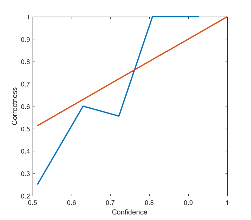
But what if we looked at real functions? If we use a single function $f(x,y)$ the zeros will typically form a curve in the plane. In order to get discrete zeros we typically need to have two functions to produce a zero set. We can think of it as a map from R2 to R2 $F(x)=[f_1(x_1,x_2), f_2(x_1,x_2)]$ where the x’es are 2D vectors. In this case Newton’s method turns into solving the linear equation system $J(x_n)(x_{n+1}-x_n)=-F(x_n)$ where $J(x_n)$ is the Jacobian matrix ( $J_{ij}=dF_i/dx_j$ ) and $x_n$ now denotes the n’th iterate.

The simplest case of nontrivial dynamics of the method is for third degree polynomials, and we want the x- and y-directions to interact a bit, so a first try is $F=[x^3-x-y, y^3-x-y]$ . Below is a plot of the first and second components (red and green), as well as a blue plane for zero values. The zeros of the function are the three points where red, green and blue meet.

We have three zeros, one at $x=y=-\sqrt{2}$ , one at $x=y=0$ , and one at $x=y=\sqrt{2}.$ The middle one has a region of troublesomely similar function values – the red and green surfaces are tangent there.

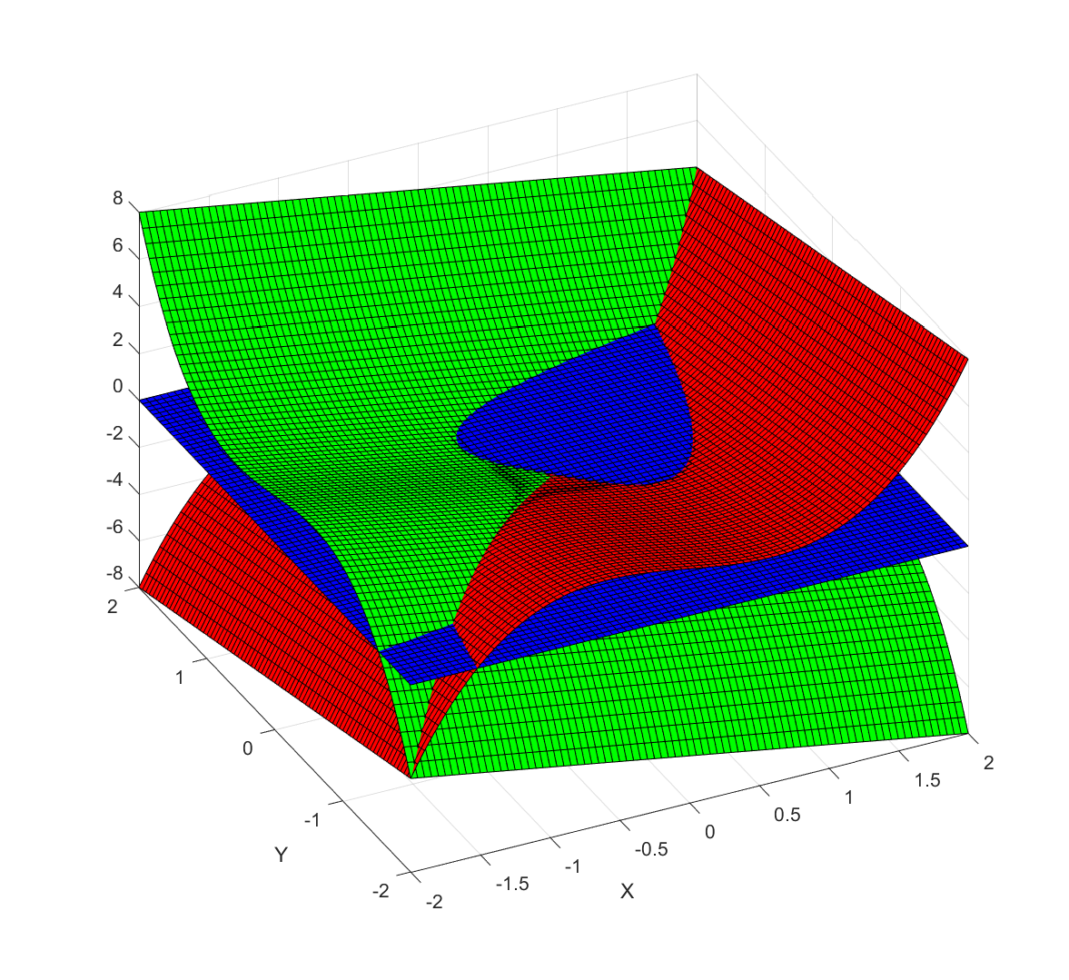
Plot of x^3-x-y (red), y^3-x-y (green) and z=0 (blue). The zeros found using Newton's method are the points where red, green and blue meet. — Plot of x^3-x-y (red), y^3-x-y (green) and z=0 (blue). The zeros found using Newton’s method are the points where red, green and blue meet.

The resulting fractal has a decided modernist bent to it, all hyperbolae and swooshes:

Behavior of Newton's method in 2D for F=[x^3-x-y, y^3-x-y]. Color denotes value of x+y, with darkening for slow convergence. — Behavior of Newton’s method in 2D for F=[x^3-x-y, y^3-x-y]. Color denotes value of x+y, with darkening for slow convergence.

The troublesome region shows up, as well as the red and blue regions where iterates run off to large or small values: the three roots are green shades.

Why is the style modernist?

In complex iterations you typically multiply with complex numbers, and if they have an imaginary component (they better have, to be complex!) that introduces a rotation or twist. Hence baroque filaments are ubiquitous, and you get the typical complex “style”.

But here we are essentially multiplying with a real matrix. For a real 2×2 matrix to be a rotation matrix it has to have a pair of imaginary eigenvalues, and for it to at least twist things around the trace needs to be small enough compared to the determinant so that there are complex eigenvalues: $T^2/4<D$ (where $T=a+d$ and $D=ad-bc$ if the matrix has the usual $[a b; c d]$ form). So if the trace and determinant are randomly chosen, we should expect a majority of cases to be non-rotational.

Moreover, in this particular case, the Jacobian tends to be diagonally dominant (quadratic terms on the diagonal) and that makes the inverse diagonally dominant too: the trace will be big, and hence the chance of seeing rotation goes down even more. The two “knots” where a lot of basins of attraction come together are the points where the trace does vanish, but since the Jacobian is also symmetric there will not be any rotation anyway. Double guarantee.

Can we make a twisty real Newton fractal? If we start with a vanilla rotation matrix and try to find a function that produces it the simplest case is $F=[x \cos(\theta) + y \sin(\theta), x\sin(\theta)+y\cos(\theta)]$ . This is of course just a rotation by the angle theta, and it does not have very interesting zeros.

To get something fractal we need more zeros, and a few zeros in the derivatives too (why? because they cause iterates to be thrown away far from where they were, ensuring a complicated structure of the basin boundaries). One attempt is $F=[ (x^3-x-y) \cos(\theta)$ $-(y^3-x-y) \sin(\theta),$ $(x^3-x-y) \sin(\theta)+(y^3-y-x) \cos(\theta) ]$ . The result is fun, but still far from baroque:

Basins of attraction for Netwon's method of twisted cubic. theta=1. — Basins of attraction for Netwon’s method of twisted cubic. theta=1.

Basins of attraction for Netwon's method of twisted cubic. theta=0.1. — Basins of attraction for Netwon’s method of twisted cubic. theta=0.1.

The problem might be that the twistiness is not changing. So we can make $\theta=x$ to make the dynamics even more complex:

Basins of attraction with rotation proportional to x.

Quite lovely, although still not exactly what I wanted (sounds like a Christmas present).

Back to the classics?

It might be easier just to hide the complex dynamics in an apparently real function like $F=[x^3-3xy^2-1, 3x^2y-y^3]$ (which produces the archetypal $f(z)=z^3-1$ Newton fractal).

Newton fractal for F=[x^3-3xy^2-1, 3x^2y-y^3]. Red and blue circles mark regions where iterates venture far from the origin.

It is interesting to see how much perturbing it causes a modernist shift. If we use $F=[x^3-3xy^2-1 + \epsilon x, 3x^2y-y^3]$ , then for $\epsilon=1$ we get:

Perturbed z^3-1 Newton iteration, epsilon=1.

As we make the function more perturbed, it turns more modernist, undergoing a topological crisis for epsilon between 3.5 and 4:

Perturbed z^3-1 Newton iteration, epsilon=2.

Perturbed z^3-1 Newton iteration, epsilon=3.

Perturbed z^3-1 Newton iteration, epsilon=3.5.

Perturbed z^3-1 Newton iteration, epsilon=4.

In the end, we can see that the border between classic baroque complex fractals and the modernist swooshy real fractals is fuzzy. Or, indeed, fractal.

A crazy futurist writes about crazy futurists

Warren Ellis’ Normal is a little story about the problem of being serious about the future.

As I often point out, most people in the futures game are basically in the entertainment industry: telling wonderful or frightening stories that allow us to feel part of a bigger sweep of history, reflect a bit, and then return to the present with the reassurance that we have some foresight. Relatively little future studies is about finding decision-relevant insights and then acting on it. It exists, but it is not the bulk of future-oriented people. Taking the future seriously might require colliding with your society as you try to tell it it is going the wrong way. Worse, the conclusions might tell you that your own values and goals are wrong.

Normal takes place at a sanatorium for mad futurists in the wilds of Oregon. The idea is that if you spend too much time thinking too seriously about the big and horrifying things in the future mental illness sets in. So when futurists have nervous breakdowns they get sent by their sponsors to Normal to recover. They are useful, smart, and dedicated people but since the problems they deal with are so strange their conditions are equally unusual. The protagonist arrives just in time to encounter a bizarre locked room mystery – exactly the worst kind of thing for a place like Normal with many smart and fragile minds – driving him to investigate what is going on.

As somebody working with the future, I think the caricatures of these futurists (or rather their ideas) are spot on. There are the urbanists, the singularitarians, the neoreactionaries, the drone spooks, and the invented professional divisions. Of course, here they are mad in a way that doesn’t allow them to function in society which softballs the views: singletons and Molochs are serious real ideas that should make your stomach lurch.

The real people I know who take the future seriously are overall pretty sane. I remember a documentary filmmaker at a recent existential risk conference mildly complaining that people where so cheerful and well-adapted: doubtless some darkness and despair would have made a far more compelling imagery than chummy academics trying to salvage the bioweapons convention. Even the people involved in developing the Mutually Assured Destruction doctrine seem to have been pretty healthy. People who go off on the deep end tend to do it not because of The Future but because of more normal psychological fault lines. Maybe we are not taking the future seriously enough, but I suspect it is more a case of an illusion of control: we know we are at least doing something.

This book convinced me that I need to seriously start working on my own book project, the “glass is half full” book. Much of our research at FHI seems to be relentlessly gloomy: existential risk, AI risk, all sorts of unsettling changes to the human condition that might slurp us down into a valueless attractor asymptoting towards the end of time. But that is only part of it: there are potential futures so bright that we do not just need sunshades, but we have problems with even managing the positive magnitude in an intellectually useful way. The reason we work on existential risk is that we (1) think there is enormous positive potential value at stake, and (2) we think actions can meaningfully improve chances. That is no pessimism, quite the opposite. I can imagine Ellis or one of his characters skeptically looking at me across the table at Normal and accusing me of solutionism and/or a manic episode. Fine. I should lay out my case in due time, with enough logos, ethos and pathos to convince them (Muhahaha!).

I think the fundamental horror at the core of Normal – and yes, I regard this more as a horror story than a techno-thriller or satire – is the belief that The Future is (1) pretty horrifying and (2) unstoppable. I think this is a great conceit for a story and a sometimes necessary intellectual tonic to consider. But it is bad advice for how to live a functioning life or actually make a saner future.

Some appearances

Two recordings of me:

First, Podcast with John Danaher, for his Algocracy project, about time acceleration in computing and the social and ethical issues this raises.

Second, a panel with me, Olle Häggström, Eva-Lotta Grantén and moderated by Carl Reinhold Bråkenhielm talking (in Swedish) at a Cusanus workshop about “Transhumanism – tekniken som frälsningsväg”:

Settling Titan, Schneier’s Law, and scenario thinking

Charles Wohlforth and Amanda R. Hendrix want us to colonize Titan. The essay irritated me in an interesting manner.

Full disclosure: they interviewed me while they were writing their book Beyond Earth: Our Path to a New Home in the Planets, which I have not read yet, and I will only be basing the following on the SciAm essay. It is not really about settling Titan either, but something that bothers me with a lot of scenario-making.

A weak case for Titan and against Luna and Mars

Basically the essay outlines reasons why other locations in the solar system are not good: Mercury too hot, Venus way too hot, Mars and Luna have too much radiation. Only Titan remains, with a cold environment but not too much radiation.

A lot of course hinges on the assumptions:

We expect human nature to stay the same. Human beings of the future will have the same drives and needs we have now. Practically speaking, their home must have abundant energy, livable temperatures and protection from the rigors of space, including cosmic radiation, which new research suggests is unavoidably dangerous for biological beings like us.

I am not that confident in that we will remain biological or vulnerable to radiation. But even if we decide to accept the assumptions, the case against the Moon and Mars is odd:

Practically, a Moon or Mars settlement would have to be built underground to be safe from this radiation.Underground shelter is hard to build and not flexible or easy to expand. Settlers would need enormous excavations for room to supply all their needs for food, manufacturing and daily life.

So making underground shelters is much harder than settling Titan, where buildings need to be isolated against a -179 C atmosphere and ice ground full with complex and quite likely toxic hydrocarbons. They suggest that there is no point in going to the moon to live in an underground shelter when you can do it on Earth, which is not too unreasonable – but is there a point in going to live inside an insulated environment on Titan either? The actual motivations would likely be less of a desire for outdoor activities and more scientific exploration, reducing existential risk, and maybe industrialization.

Also, while making underground shelters in space may be hard, it does not look like an insurmountable problem. The whole concern is a bit like saying submarines are not practical because the cold of the depths of the ocean will give the crew hypothermia – true, unless you add heating.

I think this is similar to Schneier’s law:

Anyone, from the most clueless amateur to the best cryptographer, can create an algorithm that he himself can’t break.

It is not hard to find a major problem with a possible plan that you cannot see a reasonable way around. That doesn’t mean there isn’t one.

Settling for scenarios

Maybe Wohlforth and Hendrix spent a lot of time thinking about lunar excavation issues and consistent motivations for settlements to reach a really solid conclusion, but I suspect that they came to the conclusion relatively lightly. It produces an interesting scenario: Titan is not the standard target when we discuss where humanity ought to go, and it is an awesome environment.

Similarly the “humans will be humans” scenario assumptions were presumably chosen not after a careful analysis of relative likelihood of biological and postbiological futures, but just because it is similar to the past and makes an interesting scenario. Plus human readers like reading about humans rather than robots. All together it makes for a good book.

Clearly I have different priors compared to them on the ease and rationality of Lunar/Martian excavation and postbiology. Or even giving us D. radiodurans genes.

In The Age of Em Robin Hanson argues that if we get the brain emulation scenario space settlement will be delayed until things get really weird: while postbiological astronauts are very adaptable, so much of the mainstream of civilization will be turning inward towards a few dense centers (for economics and communications reasons). Eventually resource demand, curiosity or just whatever comes after the Age of Ems may lead to settling the solar system. But that process will be pretty different even if it is done by mentally human-like beings that do need energy and protection. Their ideal environments would be energy-gradient rich, with short communications lags: Mercury, slowly getting disassembled into a hot Dyson shell, might be ideal. So here the story will be no settlement, and then wildly exotic settlement that doesn’t care much about the scenery.

But even with biological humans we can imagine radically different space settlement scenarios, such as the Gerhard O’Neill scenario where planetary surfaces are largely sidestepped for asteroids and space habitats. This is Jeff Bezo’s vision rather than Elon Musk’s and Wohlforth/Hendrix’s. It also doesn’t tell the same kind of story: here our new home is not in the planets but between them.

My gripe is not against settling Titan, or even thinking it is the best target because of some reasons. It is against settling too easily for nice scenarios.

Beyond the good story

Sometimes we settle for scenarios because they tell a good story. Sometimes because they are amenable to study among other, much less analyzable possibilities. But ideally we should aim at scenarios that inform us in a useful way about options and pathways we have.

That includes making assumptions wide enough to cover relevant options, even the less glamorous or tractable ones.

That requires assuming future people will be just as capable (or more) at solving problems: just because I can’t see a solution to X doesn’t mean it is not trivially solved in the future.

(Maybe we could call it the “Manure Principle” after the canonical example of horse manure being seen as a insoluble urban planning problem at the previous turn of century and then neatly getting resolved by unpredicted trams and cars – and just like Schneier’s law and Stigler’s law the reality is of course more complex than the story.)

In standard scenario literature there are often admonitions not just to select a “best case scenario”, “worst case scenario” and “business as usual scenario” – scenario planning comes into its own when you see nontrivial, mixed value possibilities. In particular, we want decision-relevant scenarios that make us change what we will do when we hear about them (rather than good stories, which entertain but do not change our actions). But scenarios on their own do not tell us how to make these decisions: they need to be built from our rationality and decision theory applied to their contents. Easy scenarios make it trivial to choose (cake or death?), but those choices would have been obvious even without the scenarios: no forethought needed except to bring up the question. Complex scenarios force us to think in new ways about relevant trade-offs.

The likelihood of complex scenarios is of course lower than simple scenarios (the conjunction fallacy makes us believe much more in rich stories). But if they are seen as tools for developing decisions rather than information about the future, then their individual probability is less of an issue.

In the end, good stories are lovely and worth having, but for thinking and deciding carefully we should not settle for just good stories or the scenarios that feel neat.

Solomon’s frozen judgement

A girl dying of cancer wanted to use cryonic preservation to have a chance at being revived in the future. While supported by her mother the father disagreed; in a recent high court ruling, the judge found that she could be cryopreserved.

As the judge noted, the verdict was not a statement on the validity of cryonics itself, but about how to make decisions about prospective orders. In many ways the case would presumably have gone the same way if there had been a disagreement about whether the daughter could have catholic last rites. However, cryonics makes things fresh and exciting (I have been in the media all day thanks to this).

What is the ethics of parents disagreeing about the cryosuspension of their child?

Best interests

One obvious principle is that parents ought to act in the best interest of their children.

If the child is morally mature and with informed consent, then they can clearly have a valid interest in taking a chance on cryonics: they might not be legally adult, but as in normal medical ethics their stated interests have strong weight. Conversely, one could imagine a case where a child would not want to be preserved, in which case I think most people would agree their preferences should dominate.

The general legal consensus in the West is that the child’s welfare is so important that it can overrule the objections of parents. In UK law parents have the right and the duty to give consent for a minor. Children can consent for medical treatment, overriding their parents, at 16. However, if refusing treatment parents and court can override. This mostly comes into play in cases such as avoiding blood transfusions for religious reasons.

In this case the issue was that the parents were disagreeing and the child was not legally old enough.

If one thinks cryonics is reasonable, then one should clearly cryosuspend the child: it is in their best interest. But if one thinks cryonics is not reasonable, is it harming the interest of the child? This seems to require some theory of how cryonics is bad for the interests of the child.

As an analogy, imagine a case where one parent is a Jehovah’s Witness and want to refuse a treatment involving blood transfusion: the child will die without the treatment, and it will be a close call even with it. Here the objecting parent may claim that undergoing the transfusion harms the child in an important spiritual way and refuse consent. The other parent disagrees. Here the law would come down on the side of the pro-transfusion parent.

On this account and if we agree the cases are similar, we might say that parents have a legal duty to consent to cryonics.

Weak and strong reasons

In practice the controversialness of cryonics may speak against this: many people disagree about cryonics being good for one’s welfare. However, most such arguments usually seem to be based on various farfetched scenarios about how the future could be a bad place to end up in. Others bring up loss of social connections or that personal identity would be disrupted. A more rational argument is that it is an unproven treatment of dubious efficacy, which would make it irrational to undertake if there was an alternative; however since there isn’t any alternative this argument has little power. The same goes for the risk of loss of social connection or identity: had there been an alternative to death (which definitely severs connections and dissolves identity) that may have been preferable. If one seriously thinks that the future would be so dark that it is better not to get there, one should probably not have children.

In practice it is likely that the status of cryonics as nonstandard treatment would make the law hesitate to overrule parents. We know blood transfusions work, and while spiritual badness might be a respectable as a private view we as a society do not accept it as a sufficient reason to have somebody die. But in the case of cryonics the unprovenness of the treatment means that hope for revival is on nearly the same epistemic level as spiritual badness: a respectable private view, but not strong enough to be a valid public reason. Cryonicists are doing their best to produce scientific evidence – tissue scans, memory experiments, protocols – that move the reasons to believe in cryonics from the personal faith level to the public evidence level. They already have some relevant evidence. As soon as lab mice are revived or people become convinced the process saves the connectome the reasons would be strengthened and cryonics becomes more akin blood transfusion.

The key difference is that weak private reasons are enough to allow an experimental treatment where there is no alternative but death, but they are generally not enough to go for an experimental treatment when there is some better treatment. When disallowing a treatment weak reasons may work well against unproven or uncertain treatments, but not when it is proven. However, disallowing a treatment with no alternative is equivalent to selecting death.

When two parents disagree about cryonics (and the child does not have a voice) it hence seems that they both have weak reasons, but the asymmetry between having a chance and dying tilts in favor of cryonics. If it was purely a matter of aesthetics or value (for example, arguing about the right kind of last rites) there would be no societal or ethical constraint. But here there is some public evidence, making it at least possible that the interests of the child might be served by cryonics. Better safe than sorry.

When the child also has a voice and can express its desires, then it becomes obvious which way to go.

King Solomon might have solved the question by cryosuspending the child straight away, promising the dissenting parent not to allow revival until they either changed their mind or there was enough public evidence to convince anybody that it would be in the child’s interest to be revived. The nicest thing about cryonics is that it buys you time to think things through.

AI, morality, ethics and metaethics

Next Sunday I will be debating AI ethics at Battle of Ideas. Here is a podcast where I talk AI, morality and ethics: https://soundcloud.com/institute-of-ideas/battle-cry-anders-sandberg-on-ethical-ai

What distinguishes morals from ethics?

There is actually a shocking confusion about what the distinction between morals and ethics is. Differen.com says ethics is about rules of conduct produced by an external source while morals are an individual’s own principles of right and wrong. Grammarist.com says morals are principles on which one’s own judgement of right and wrong are based (abstract, subjective and personal), ethics are the principles of right conduct (practical, social and objective). Ian Welsh gives a soundbite: “morals are how you treat people you know. Ethics are how you treat people you don’t know.” Paul Walker and Terry Lovat say ethics leans towards decisions based on individual character and subjective understanding of right and wrong, while morals is about widely shared communal or societal norms – here ethics is individual assessment of something being good or bad, while morality is inter-subjective community assessment.

Wikipedia distinguishes between ethics as a research field and the common human ability to think critically about moral values and direct actions appropriately, or a particular persons principles of values. Morality is the differentiation between things that are proper and improper, as well as a body of standards and principles in derived from a code of conduct in some philosophy, religion or culture… or derived from a standard a person believes to be universal.

Dictionary.com regards ethics as a system of moral principles, the rules of conduct recognized in some human environment, an individual’s moral principles (and the branch of philosophy). Morality is about conforming to the rules of right conduct, having moral quality or character, a doctrine or system of morals and a few other meanings. The Cambridge dictionary thinks ethics is the study of what is right or wrong, or the set of beliefs about it, while morality is a set of personal or social standards for good/bad behavior and character.

And so on.

I think most people try to include the distinction between shared systems of conduct and individual codes, and the distinction between things that are subjective, socially agreed on, and maybe objective. Plus that we all agree on that ethics is a philosophical research field.

My take on it

I like to think of it as a AI issue. We have a policy function $\pi(s,a)$ that maps states and action pairs to a probability of acting that way; this is set using a value function $Q(s)$ where various states are assigned values. Morality in my sense is just the policy function and maybe the value function: they have been learned through interacting with the world in various ways.

Ethics in my sense is ways of selecting policies and values. We are able to not only change how we act but also how we evaluate things, and the information that does this change is not just reward signals that update value function directly, but also knowledge about the world, discoveries about ourselves, and interactions with others – in particular ideas that directly change the policy and value functions.

When I realize that lying rarely produces good outcomes (too much work) and hence reduce my lying, then I am doing ethics (similarly, I might be convinced about this by hearing others explain that lying is morally worse than I thought or convincing me about Kantian ethics). I might even learn that short-term pleasure is less valuable than other forms of pleasure, changing how I view sensory rewards.

Academic ethics is all about the kinds of reasons and patterns we should use to update our policies and values, trying to systematize them. It shades over into metaethics, which is trying to understand what ethics is really about (and what metaethics is about: it is its own meta-discipline, unlike metaphysics that has metametaphysics, which I think is its own meta-discipline).

I do not think I will resolve any confusion, but at least this is how I tend to use the terminology. Morals is how I act and evaluate, ethics is how I update how I act and evaluate, metaethics is how I try to think about my ethics.

How much should we spread out across future scenarios?

Robin Hanson mentions that some people take him to task for working on one scenario (WBE) that might not be the most likely future scenario (“standard AI”); he responds by noting that there are perhaps 100 times more people working on standard AI than WBE scenarios, yet the probability of AI is likely not a hundred times higher than WBE. He also notes that there is a tendency for thinkers to clump onto a few popular scenarios or issues. However:

In addition, due to diminishing returns, intellectual attention to future scenarios should probably be spread out more evenly than are probabilities. The first efforts to study each scenario can pick the low hanging fruit to make faster progress. In contrast, after many have worked on a scenario for a while there is less value to be gained from the next marginal effort on that scenario.

This is very similar to my own thinking about research effort. Should we focus on things that are likely to pan out, or explore a lot of possibilities just in case one of the less obvious cases happens? Given that early progress is quick and easy, we can often get a noticeable fraction of whatever utility the topic has by just a quick dip. The effective altruist heuristic of looking at neglected fields also is based on this intuition.

A model

But under what conditions does this actually work? Here is a simple model:

There are $N$ possible scenarios, one of which ( $j$ ) will come about. They have probability $P_i$ . We allocate a unit budget of effort to the scenarios: $\sum a_i = 1$ . For the scenario that comes about, we get utility $\sqrt{a_j}$ (diminishing returns).

Here is what happens if we allocate proportional to a power of the scenarios, $a_i \propto P_i^\alpha$ . $\alpha=0$ corresponds to even allocation, 1 proportional to the likelihood, >1 to favoring the most likely scenarios. In the following I will run Monte Carlo simulations where the probabilities are randomly generated each instantiation. The outer bluish envelope represents the 95% of the outcomes, the inner ranges from the lower to the upper quartile of the utility gained, and the red line is the expected utility.

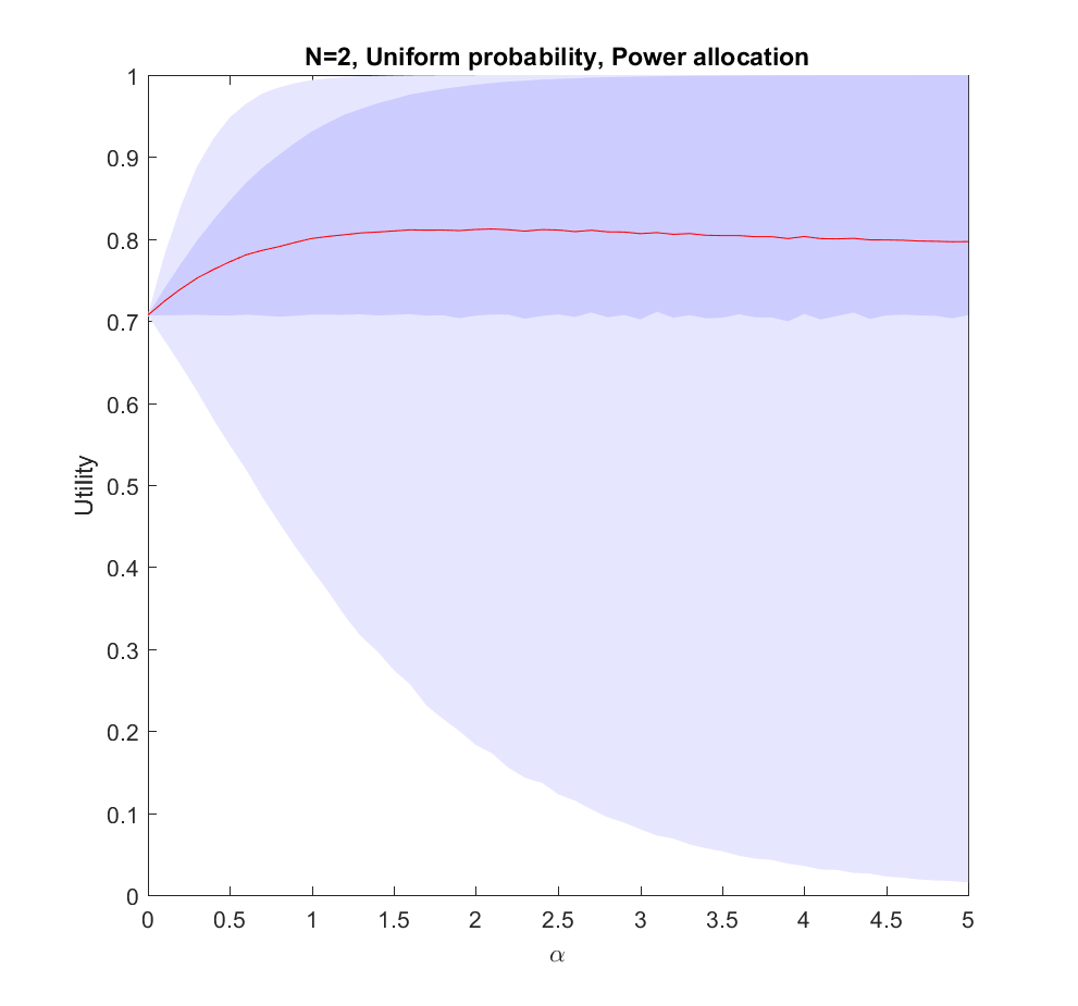
Utility of allocating effort as a power of the probability of scenarios. Red line is expected utility, deeper blue envelope is lower and upper quartiles, lighter blue 95% interval.

This is the $N=2$ case: we have two possible scenarios with probability $p$ and $1-p$ (where $p$ is uniformly distributed in [0,1]). Just allocating evenly gives us $1/\sqrt{2}$ utility on average, but if we put in more effort on the more likely case we will get up to 0.8 utility. As we focus more and more on the likely case there is a corresponding increase in variance, since we may guess wrong and lose out. But 75% of the time we will do better than if we just allocated evenly. Still, allocating nearly everything to the most likely case means that one does lose out on a bit of hedging, so the expected utility declines slowly for large $\alpha$ .

The $N=100$ case (where the probabilities are allocated based on a flat Dirichlet distribution) behaves similarly, but the expected utility is smaller since it is less likely that we will hit the right scenario.

What is going on?

This doesn’t seem to fit Robin’s or my intuitions at all! The best we can say about uniform allocation is that it doesn’t produce much regret: whatever happens, we will have made some allocation to the possibility. For large N this actually works out better than the directed allocation for a sizable fraction of realizations, but on average we get less utility than betting on the likely choices.

The problem with the model is of course that we actually know the probabilities before making the allocation. In reality, we do not know the likelihood of AI, WBE or alien invasions. We have some information, and we do have priors (like Robin’s view that $P_{AI} < 100 P_{WBE}$ ), but we are not able to allocate perfectly. A more plausible model would give us probability estimates instead of the actual probabilities.

We know nothing

Let us start by looking at the worst possible case: we do not know what the true probabilities are at all. We can draw estimates from the same distribution – it is just that they are uncorrelated with the true situation, so they are just noise.

Utility of allocating effort as a power of the probability of scenarios, but the probabilities are just random guesses. Red line is expected utility, deeper blue envelope is lower and upper quartiles, lighter blue 95% interval. 100 possible scenarios, with uniform probability on the simplex.

In this case uniform distribution of effort is optimal. Not only does it avoid regret, it has a higher expected utility than trying to focus on a few scenarios ( $\alpha>0$ ). The larger N is, the less likely it is that we focus on the right scenario since we know nothing. The rationality of ignoring irrelevant information is pretty obvious.

Note that if we have to allocate a minimum effort to each investigated scenario we will be forced to effectively increase our $\alpha$ above 0. The above result gives the somewhat optimistic conclusion that the loss of utility compared to an even spread is rather mild: in the uniform case we have a pretty low amount of effort allocated to the winning scenario, so the low chance of being right in the nonuniform case is being balanced by having a slightly higher effort allocation on the selected scenarios. For high $\alpha$ there is a tail of rare big “wins” when we hit the right scenario that drags the expected utility upwards, even though in most realizations we bet on the wrong case. This is very much the hedgehog predictor story: ocasionally they have analysed the scenario that comes about in great detail and get intensely lauded, despite looking at the wrong things most of the time.

We know a bit

We can imagine that knowing more should allow us to gradually interpolate between the different results: the more you know, the more you should focus on the likely scenarios.

Optimal alpha as a function of how much information we have about the true probabilities. N=2. — Optimal alpha as a function of how much information we have about the true probabilities (noise due to Monte Carlo and discrete steps of alpha). N=2 (N=100 looks similar).

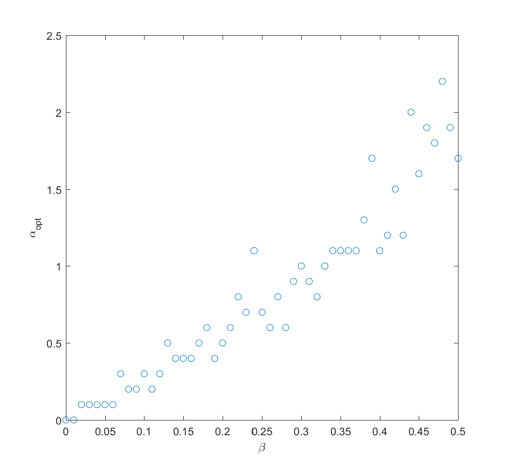
If we take the mean of the true probabilities with some randomly drawn probabilities (the “half random” case) the curve looks quite similar to the case where we actually know the probabilities: we get a maximum for $\alpha\approx 2$ . In fact, we can mix in just a bit ( $\beta$ ) of the true probability and get a fairly good guess where to allocate effort (i.e. we allocate effort as $a_i \propto (\beta P_i + (1-\beta)Q_i)^\alpha$ where $Q_i$ is uncorrelated noise probabilities). The optimal alpha grows roughly linearly with $\beta$ , $\alpha_{opt} \approx 4\beta$ in this case.

We learn

Adding a bit of realism, we can consider a learning process: after allocating some effort $\gamma$ to the different scenarios we get better information about the probabilities, and can now reallocate. A simple model may be that the standard deviation of noise behaves as $1/\sqrt{\tilde{a}_i}$ where $\tilde{a}_i$ is the effort placed in exploring the probability of scenario $i$ . So if we begin by allocating uniformly we will have noise at reallocation of the order of $1/\sqrt{\gamma/N}$ . We can set $\beta(\gamma)=\sqrt{\gamma/N}/C$ , where $C$ is some constant denoting how tough it is to get information. Putting this together with the above result we get $\alpha_{opt}(\gamma)=\sqrt{2\gamma/NC^2}$ . After this exploration, now we use the remaining $1-\gamma$ effort to work on the actual scenarios.

Expected utility as a function of amount of probability-estimating effort (gamma) for C=1 (hard to update probabilities), C=0.1 and C=0.01 (easy to update). N=100.

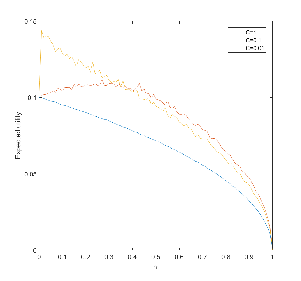
This is surprisingly inefficient. The reason is that the expected utility declines as $\sqrt{1-\gamma}$ and the gain is just the utility difference between the uniform case $\alpha=0$ and optimal $\alpha_{opt}$ , which we know is pretty small. If C is small (i.e. a small amount of effort is enough to figure out the scenario probabilities) there is an optimal nonzero $\gamma$ . This optimum $\gamma$ decreases as C becomes smaller. If C is large, then the best approach is just to spread efforts evenly.

Conclusions

So, how should we focus? These results suggest that the key issue is knowing how little we know compared to what can be known, and how much effort it would take to know significantly more.

If there is little more that can be discovered about what scenarios are likely, because our state of knowledge is pretty good, the world is very random, or improving knowledge about what will happen will be costly, then we should roll with it and distribute effort either among likely scenarios (when we know them) or spread efforts widely (when we are in ignorance).

If we can acquire significant information about the probabilities of scenarios, then we should do it – but not overdo it. If it is very easy to get information we need to just expend some modest effort and then use the rest to flesh out our scenarios. If it is doable but costly, then we may spend a fair bit of our budget on it. But if it is hard, it is better to go directly on the object level scenario analysis as above. We should not expect the improvement to be enormous.

Here I have used a square root diminishing return model. That drives some of the flatness of the optima: had I used a logarithm function things would have been even flatter, while if the returns diminish more mildly the gains of optimal effort allocation would have been more noticeable. Clearly, understanding the diminishing returns, number of alternatives, and cost of learning probabilities better matters for setting your strategy.

In the case of future studies we know the number of scenarios are very large. We know that the returns to forecasting efforts are strongly diminishing for most kinds of forecasts. We know that extra efforts in reducing uncertainty about scenario probabilities in e.g. climate models also have strongly diminishing returns. Together this suggests that Robin is right, and it is rational to stop clustering too hard on favorite scenarios. Insofar we learn something useful from considering scenarios we should explore as many as feasible.